1,306
Views
9
CrossRef citations to date
0
Altmetric
Soil physics

A seasonal behavior of surface soil moisture condition in a reclaimed tropical peatland

, &
Pages 543-552 | Received 26 Jan 2012, Accepted 18 Aug 2012, Published online: 02 Nov 2012

Figures & data

Table 1. Physical properties found in the soil layers in the study site. The top layer (0–60 cm in depth) was more brightly colored with smaller amount of organic matter content and higher bulk density

Figure 1. Seasonal behaviors of (a) precipitation, (b) volumetric water content at 5 cm in depth, and (c) groundwater level relative to the land surface from March 2010 to November 2011.
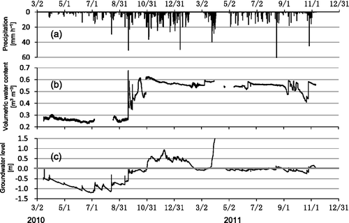
Figure 1. Seasonal behaviors of (a) precipitation, (b) volumetric water content at 5 cm in depth, and (c) groundwater level relative to the land surface from March 2010 to November 2011.

Figure 2. (a) Shows the plots from the triplicate k(h) measurements for the soil samples taken from the top 60-cm layer while the solid line, the dotted line, and the chain line denote the modeled curves of k(h) = ks /(1 + h/a) with ks  = 6 × 10−4, 3 × 10−2 and 3 × 10−5  cm s−1, respectively. The parameter a = −0.04 is consistently used. (b) Soil water retention curves obtained from the k(h) measurements (△) and from the hanging-water-column (HWC) and the pressure-plate (PP) methods (▪). Horizontal bars attached to the plots of △ denote the one standard error below and above the data plots among the h values recorded by the five tensiometers. Vertical bars drawn on the plots of ▪ indicate one standard error below and above the data plots for the triplicates of the HWC and the PP methods. The dotted line is the van Genuchten model θ = θr  + (θ sθr )(1 + α|h| n )−1+1/ n (van Genuchten Citation1980) with the parameters of θ s = 0.63 m3 m−3, θr  = 0.26 m3 m−3, α = 0.01, and n = 1.4.
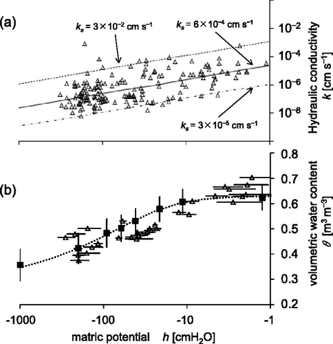
Figure 2. (a) Shows the plots from the triplicate k(h) measurements for the soil samples taken from the top 60-cm layer while the solid line, the dotted line, and the chain line denote the modeled curves of k(h) = ks /(1 + h/a) with ks  = 6 × 10−4, 3 × 10−2 and 3 × 10−5  cm s−1, respectively. The parameter a = −0.04 is consistently used. (b) Soil water retention curves obtained from the k(h) measurements (△) and from the hanging-water-column (HWC) and the pressure-plate (PP) methods (▪). Horizontal bars attached to the plots of △ denote the one standard error below and above the data plots among the h values recorded by the five tensiometers. Vertical bars drawn on the plots of ▪ indicate one standard error below and above the data plots for the triplicates of the HWC and the PP methods. The dotted line is the van Genuchten model θ = θr  + (θ s−θr )(1 + α|h| n )−1+1/ n (van Genuchten Citation1980) with the parameters of θ s = 0.63 m3 m−3, θr  = 0.26 m3 m−3, α = 0.01, and n = 1.4.

Figure 3. The θ 5cm–GWL relation based on the measured data sets on . Symbols of circle (○) and plus (+) denote the plots obtained while the groundwater table was going downward and upward, respectively. Solid lines show the simulated curves based on Equation (Equation4) with the parameters specified in . The upward water flux E in Equation (Equation4) was varied from 2 to 4, 6 and 8 mm d−1. The simulated curves were extrapolated into the matric potential domain of h < −1000 cm where the k(h) was not measured (dotted lines), and were terminated at GWL = −60 cm since both the k(h) and the θ(h) were evaluated only for the top 60 cm layer.
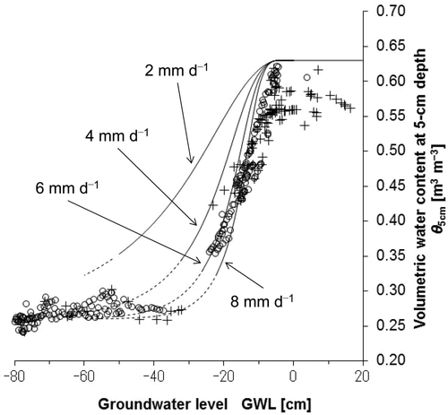
Figure 3. The θ 5cm–GWL relation based on the measured data sets on Fig. 1. Symbols of circle (○) and plus (+) denote the plots obtained while the groundwater table was going downward and upward, respectively. Solid lines show the simulated curves based on Equation (Equation4) with the parameters specified in Fig. 2a. The upward water flux E in Equation (Equation4) was varied from 2 to 4, 6 and 8 mm d−1. The simulated curves were extrapolated into the matric potential domain of h < −1000 cm where the k(h) was not measured (dotted lines), and were terminated at GWL = −60 cm since both the k(h) and the θ(h) were evaluated only for the top 60 cm layer.

Figure 4. (a) The sensitivity of the h 5cm–GWL relation to the modeled k(h) curve. The three modeled k(h) curves displayed in were used. The upward water flux E of 6 mm d−1 was consistently adopted in all three simulations. (b) The transition of the h 5cm–GWL relation with varying the upward water flux E. All three curves share the same k(h) = ks /(1 + h/a) with ks  = 6 × 10−4 cm s–1 and a = –0.04, and the chain line denotes E = 10 mm d–1 while the two-dot chain line represents E = 2 mm d–1.
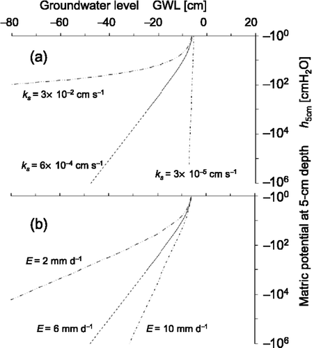
Figure 4. (a) The sensitivity of the h 5cm–GWL relation to the modeled k(h) curve. The three modeled k(h) curves displayed in Fig. 2a were used. The upward water flux E of 6 mm d−1 was consistently adopted in all three simulations. (b) The transition of the h 5cm–GWL relation with varying the upward water flux E. All three curves share the same k(h) = ks /(1 + h/a) with ks  = 6 × 10−4 cm s–1 and a = –0.04, and the chain line denotes E = 10 mm d–1 while the two-dot chain line represents E = 2 mm d–1.

Reprints and Corporate Permissions

Please note: Selecting permissions does not provide access to the full text of the article, please see our help page How do I view content?

To request a reprint or corporate permissions for this article, please click on the relevant link below:

Academic Permissions

Please note: Selecting permissions does not provide access to the full text of the article, please see our help page How do I view content?

Obtain permissions instantly via Rightslink by clicking on the button below:

If you are unable to obtain permissions via Rightslink, please complete and submit this Permissions form. For more information, please visit our Permissions help page.