Pore rigidity in structured soils—only a theoretical boundary condition for hydraulic properties?

Figures & data

Table 1 Physical (grain size distribution, structure, and bulk density ρt) and organic matter of all investigated sites/soil horizons. Soil types are defined according to IUSS/ISRIC/FAO (2006) and texture are defined according to the German classification system (Boden 2005). Wacken, Ritzerau, Hildesheim are locations in Germany; Cudico and Pelchuquin are sites in Chile. The sampling depth corresponds to the number attached to the abbreviation; a soil depth of 6 cm was always collected

			Depth			pt	Clay	Silt	Sand	Organic matter
Soil type	Site	Horizon	(cm)	Abbreviation	Soil structure	g cm^−3	< 2µm	2–63µm	63–2000µm	%
Eroded Stagnic Luvisol derived	Ritzerau/Germany	Ap	15–31	SS-LL(15, 25)	coherent-subangularblocky	1.59	7.4	27.4	65.2	1.7
from periglacial cover beds		App*	35–41	SS-LL(35)	platy	1.73	4.3	24.5	71.2	0.9
above Weichselian glacial till		2Btg	50–56	SS-LL(50)	subangular blocky	1.68	20.4	38.6	41	0.2
(loam and sand)		3Bw	75–81	SS-LL(75)	blocky-prismatic	1.77	8.1	28.4	63.5	0.05
Haplic Gleysol from fluvioglacial Weichselian deposits	Ritzerau/Germany	Cl	40–46	GGn(40)	coherent-blocky	1.46	34.9	57.7	7.4	0.07
Haplic Stagnosol derived from periglacial cover beds above Saalian glacial till	Wacken/Germany	2Cg	50–56	SSn(50)	coherent-(blocky)	1.21	64.9	15	20.1	0.15
Haplic Chernozem derived from loess	Hildesheim/Germany	Ah	40–46	TTn(40)	subangular blocky	1.45	19.2	78.7	2.1	1.9
Rheic Histosol derived from peat above Saalian glacifluvial sands	Wacken/Germany	Hl	30–36	HNn(30)		0.81				>20
Drained Histic Gleysol derived of peatclay above Saalian glacifluvial sands	Wacken/Germany	Cl	40–46	HN-GH(40)	coherent	1.08	39.9	34.1	26	25
Humic Ultisol derived from	Cudico/Chile	Ap	5–11	US	subangular blocky	1.05	42.7	37.2	20.1	18
old volcanic ashes		Ap		UnS-1.1	coherent	1.10	42.7	37.2	20.1	18
		Ap		UnS-0.8	coherent	0.80	42.7	37.2	20.1	18
Haplic Andosol derived from volcanic ashes	Pelchuquin/Chile	Ap	5–11	A5	granular	0.69	35.3	59.5	5.2	14
		Bw	40–46	A40	subangular blocky	0.53	19.3	75.5	5.2	4

*plough pan

Figure 1 (a) Shrinkage curves of the various soil horizons of the Stagnic Luvisol (SS-LL) derived from glacial till in Northern Germany. The abbreviation is described in detail in Boden (2005). (b) Shrinkage curves of selected soil horizons of the Gleysol (GGn), Stagnosol (SSn) and Chernozem (TTn). The samples come from Northern Germany. (c) Shrinkage curves of selected soil horizons of the Haplic Andosol (A) and a Humic Ultisol (US), both under long-term pasture. Furthermore, the homogenized samples of the Humic Ultisol at a given bulk density of 1.1 or 0.8 g cm^–3 (UnS-1.1 or UnS 0.8) are shown compared to the initial structured sample (US) at the same depth of 5 cm. All samples were collected in Chile. (d) Shrinkage curves of selected soil horizons of the Rheic Histosol (HNn) and the Histic Gleysol (HN-GH), collected in northern Germany. Numbers following abbreviations define the soil depth (cm).

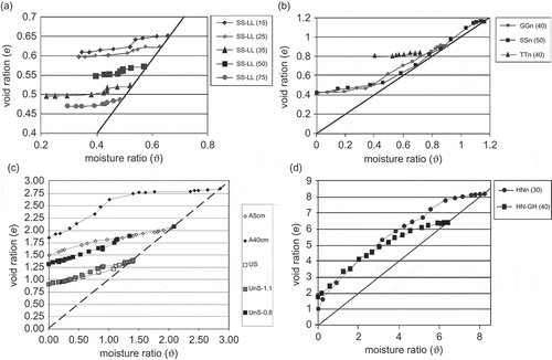
Figure 2 Relationship between void ratio and matric potential for the Stagnic Luvisol (SS-LL) Haplic Gleysol (GGn), Haplic Chernozem (TTn) and Haplic Stagnosol (SSn) collected at various sites in Germany for defined depths with varying soil structure.

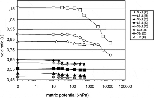
Figure 3 (a) Difference between the predicted and the actual water content due to shrinkage as a function of matric potential. (b) Difference between the predicted and the actual water content due to shrinkage as a function of matric potential for a Haplic Andisol (A) and Humic Ultisol (US), both under long-term pasture. The number following the abbreviation defines the soil depth (cm). Furthermore, the homogenized samples of the Humic Ultisol at a given bulk density of 1.1 or 0.8 g cm^–3 (UnS-1.1 or UnS 0.8) are shown compared to the initial structured sample (US) at the same depth of 5 cm.

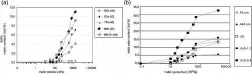
Figure 4 Effect of soil shrinkage on the pattern of the water retention curve of the Stagnosol. The differences in the water contents at a given matric potential hPa (i.e., pressure head cm) depending on the shrinkage intensity and direction are obvious. “Vertical” means that only the vertical soil shrinkage due to drying was considered, while isotropy is based on the vertically taken measurements and transferring them to three-dimensional isotropy. Anisotropy describes the actual shrinkage effects in all directions.

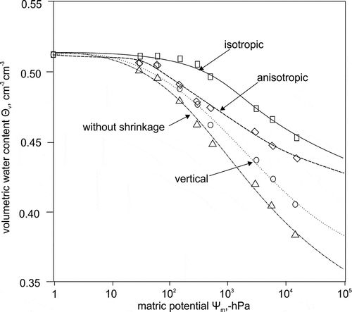
Table 2 van Genuchten parameters of the Stagnosol (SSn50) under various rigidity boundary conditions

Parameter	Without	Vertical	Isotropic	Ansiotropic 3-D
theta_r [cm^3 cm^−3]	0.22	0.29	0.41	0.41
theta_s [cm^3 cm^−3]	0.51	0.51	0.51	0.51
alpha [1 cm^–1]	0.018	0.011	0.002	0.015
n [-]	1.102	1.124	1.233	1.216
m [-]	0.092	0.110	0.189	0.178
l [-]	0.5	0.5	0.5	0.5
Ks [cm s^–1]	5.15E-06	5.15E-06	5.15E-06	5.15E-06

Ks, hydraulic conductivity (cm/s); 3-D, three-dimensional.

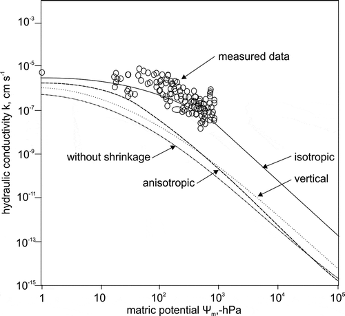
Figure 5 Hydraulic conductivity/matric potential (K/Ψm) relation of the Stagnosol derived from clay-rich till. The differences in the curve patterns depend on the measured shrinkage intensity and dimensions. “Vertical” means that only the vertical soil shrinkage due to drying was considered, while isotropy is based on the vertically taken measurements and transferring them to three dimensions. Anisotropy describes the actual shrinkage effects in all directions. The circles define actual measurements which coincide with the predicted K/Ψm curve assuming isotropy.

Blume HP, Stahr K, Leinweber P 2011: Bodenkundliches Praktikum. 3.Aufl. Spektrum Verlag, Heidelberg. ISBN: 978–3–8274–1553–0

 Google Scholar