Experimental and Numerical Analysis of a Novel Display Case Design: Case Study of the Renovated Anne Frank House

Figures & data

Figure 1. Impression of Anne Frank House exterior (left images and top right) and the interior of the new Diary room (bottom right) with display case 1. Images © Anne Frank House/Photographer: Cris Toala Olivares.

Figure 2. Floorplan of exhibition gallery with T/RH sensor locations and positions of the air in- and outlets with the air volumes involved.

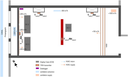
Figure 3. Sections of AHU_room and AHU_case. Image adapted from Breman.

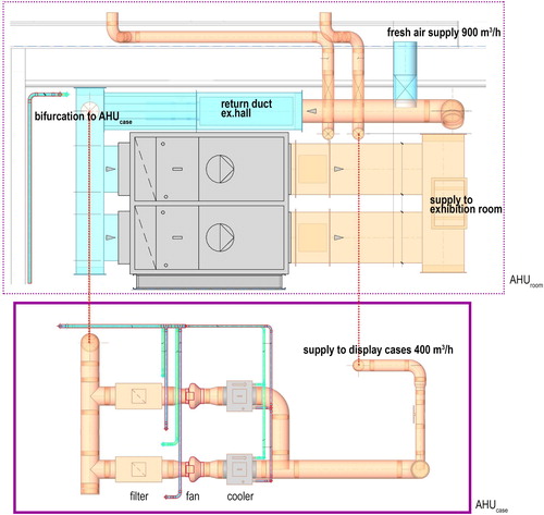
Figure 4. Simplified cross section of display case with locations of combined T/RH sensors and surface T sensors.

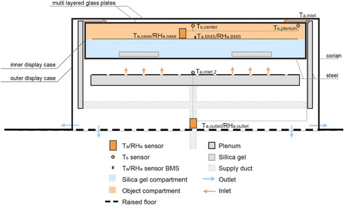
Figure 5. Photographs of Display case design while opened. Combined T/RH sensors were placed in the center of the inner display case and surface temperature sensors mounted to the inside of the glass plate.

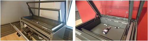
Table 1. Overview of initial parameters of experiments during this study.

Exp.	Troom [°C]	Ta,case [°C]	Ta,inlet [°C]	Duration [h]	Control setting	Objective
1	20	–	16	121.5	Tinlet control	T control performance
2	20	–	–	193	AHUcase off	malfunction test
3	20–18	18	–	1	control setting 1	emergency setting (1 h) test
4	18	–	–	1		opening of display case
5	24	–	16	122.5	Troom/Tinlet control	extreme boundary conditions test
6	20	18	–	165.5	operational control	operational use setting test
7	20–18	18	–	18	control setting 2	overnight setting (12 h) test
8	20	18	–	Continuous	RH control present	RH control performance by placement of silica gel
9	20	18	–	Continuous	RH control present	visitor influence

Figure 6. 2D model geometry of display case 1. Data point locations and dimensions in mm (right) and boundary division (right).

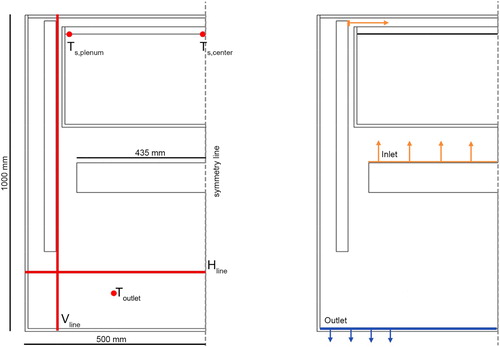
Figure 7. 3D model geometry of display case 1. Data point and data line locations (left) and dimensions in mm with boundary division (center) and surface-to-surface radiation planes (right).

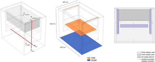
Figure 8. Coarse (left), medium (center), and fine (right) grid used for grid sensitivity analysis for the 2D and 3D cases.

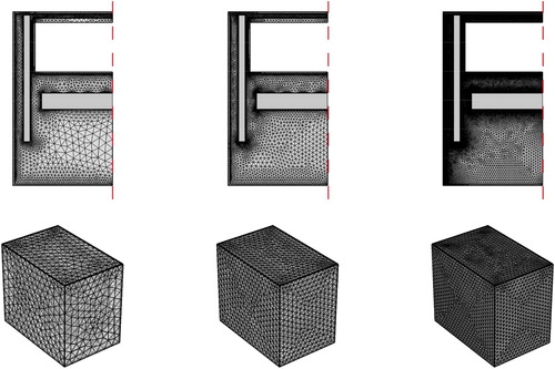
Figure 9. Outdoor temperature, relative humidity, specific humidity and irradiance of the Amsterdam location (Schiphol) during the measurement period. Starting dates of experiments are expressed by the vertical lines.

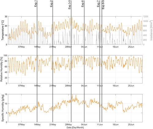
Figure 10. Comparison between T_{a, case} of the Eltek sensors (gray) and BMS sensors (orange) in display case 1 (upper), 2 (middle), and 3 (lower) during the first experiment.

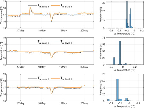
Figure 11. Indoor climate conditions of the exhibition gallery and display case 1 during experiment 1 and 2. Peak A shows a malfunction of the cooling machine and dip B shows an extra cooling capacity tests performed by the technicians.

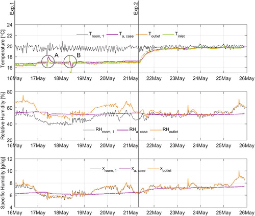
Figure 12. Indoor climate conditions of the exhibition gallery and display case 1 during experiments 3, 4, and 5. Emergency setting was tested and T_room decreased to 18°C within an hour, after which and extreme situation was imposed and T_room increased to 24°C. T_inlet was kept as close to 16°C throughout the experiment.

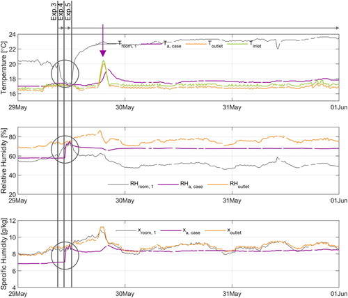
Figure 13. Indoor climate conditions of the exhibition gallery and display case 1 during experiments 7–9.

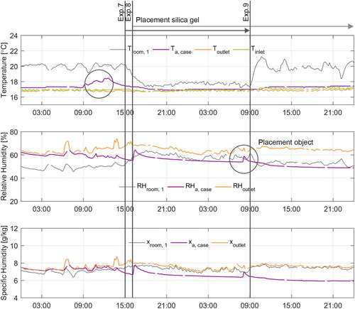
Figure 14. Indoor climate conditions of the exhibition gallery (gray) and display case (colored) during experiment 9. The exhibition gallery was opened to public during this experiment and silica gel controls RH_{a, case}.

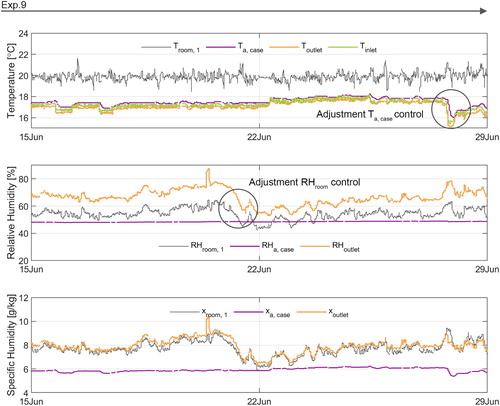
Figure 15. Grid sensitivity analysis for 2D model for T_s,center (left), T_{s, plenum}, (center) and T_outlet (right). Measurement locations can be found in Figure 6 where T_s,center, T_{s, plenum}, and T_outlet are pictured.

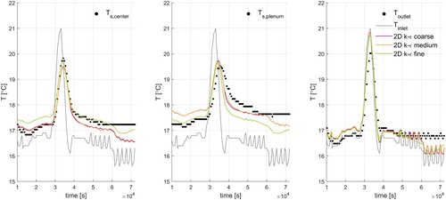
Figure 16. Grid sensitivity analysis through horizontal (left) and vertical (right) plane for 2D model. Locations of the lines can be found in Figure 6.

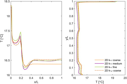
Figure 17. Comparison between experimental results and simulation results for T_s,center, (left), T_s.plenum, (center) and T_outlet (right) in the 2D and 3D case for several turbulence models.

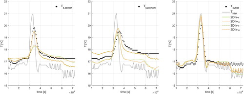
Table 2. Validation metrics for the 2D medium grid display case.

		FB			FAC 1.05			MBE			CV RMSE
		Ts,plenum	Ts,center	Toutlet	Ts,plenum	Ts,center	Toutlet	Ts,plenum	Ts,center	Toutlet	Ts,plenum	Ts,center	Toutlet
Aim		0			1			0			0
Range		(−0.3;0.3)			>0.5			<10%			<30%
2D k–ε	coarse	0.006	−0.004	0.001	1.000	1.000	1.000	0.64	0.44	0.10	7.06	4.80	1.13
	medium	0.007	−0.005	0	1.000	1.000	1.000	0.71	0.47	0.02	7.77	5.18	0.22
	fine	−0.008	−0.149	0.003	1.000	1.000	0.992	0.78	16.07	0.32	8.60	176.72	3.50
2D k–ε		0.007	−0.005	0.001	1.000	1.000	1.000	0.70	0.50	0.12	7.70	5.55	1.35
3D k–ε		0.001	0.033	0.004	0.950	0.620	1.000	0.10	3.26	0.45	1.12	35.87	4.90
3D k–ε		0.006	−0.004	0.001	1.000	1.000	1.000	0.13	3.27	0.37	1.41	35.93	4.12

Figure 18. Simulation results of yearly imposed dynamic conditioning with ASHRAE climate class AA as T_room.

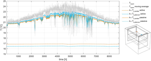
Figure A1. Indoor climate conditions of the exhibition gallery and display case 1 during experiment 6.

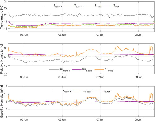
Figure A2. Imposed temperature trajectory with results (a) and comparison (b) between Eltek sensor (object) and reference sensor. The constant period is calculated (c) to provide a number of overlapping matching measurements (d).

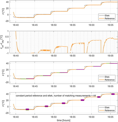
Table A1. Temperature calibration correction; average value of 44 measurements per imposed set point.

θref [°C]	θobject [°C]	θcorrection [°C]
−9.92	−8.90	−1.02
0.10	0.84	−0.74
10.10	10.50	−0.4
20.22	20.31	−0.08
30.36	30.20	0.16
39.75	39.41	0.34

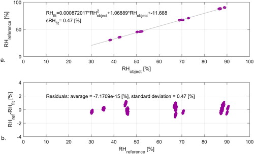
Figure A3. Eltek and reference fitting by using polynomial function (a) and the residuals to confirm the correct use of this function (b).

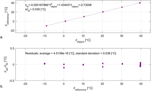
Table A2. Polynomial parameters for T and RH of the sensor used in inner display case 1.

	B2	B1	B0	sB2	sB1	sB0	1*sXfit	R^2
T	−0.00016787	1.034	−0.7301	1.1e−005	0.00037	0.0035	0.036°C	1.0
RH	0.00087202	1.0689	−11.67	6.2e−005	0.0082	0.25	0.47%	0.9995

Figure A4. Imposed relative humidity trajectory with results (a) and comparison (b) between Eltek sensor and reference sensor. The constant period is calculated (c) to provide a number of overlapping matching measurements (d).

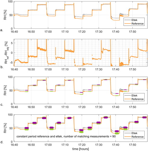
Table A3. Relative humidity calibration correction; average value per set point.

RHref [%]	RHobject [%]	RHcorrection [%]
45.20	50.30	−5.1
66.97	69.11	−2.1
88.08	86.73	1.3
46.05	51.82	−5.8
67.40	69.89	−2.5
87.79	86.92	0.87
35.43	42.50	−7.1
45.73	51.64	−5.9
67.31	70.53	−3.2
90.44	88.85	1.6
30.26	38.33	−8.1
45.98	52.10	−6.1
70.60	72.98	−2.4
90.06	89.13	0.93

Figure A5. Eltek and reference fitting by using polynomial function (a) and the residuals to confirm the correct use of this function (b).