Research and Development of a Photogrammetric Condition Monitoring Workflow to Improve Change Detection in Wall Paintings

Figures & data

Figure 1. In the tested photogrammetric monitoring workflow digital elevation models (DEM) are generated from two image blocks (referred to as epochs as they are part of a monitoring program) and are compared to create the DEM of difference (DoD) to identify and quantify change. © J. Paul Getty Trust

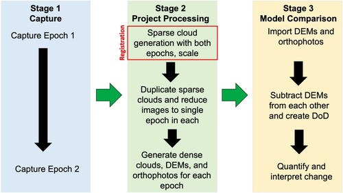
Figure 2. The steps taken to generate a three-dimensional model. Step 1: Overlapping images are captured and then imported into the photogrammetric software. Step 2: The images are processed to create a sparse cloud. Step 3: A dense cloud is generated based on the sparse cloud. Step 4: The dense cloud can then be processed into a digital elevation model (DEM) where the relative heights are represented as a heatmap. © J. Paul Getty Trust

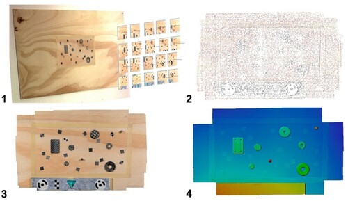
Figure 3. Patterned adhesive labels were affixed to the monitoring area to create distinct features for photogrammetric model generation (top). Objects numbered 1–8 (with the prefix H) were added to the board (bottom) and their height on the board was determined by taking and averaging measurements using a vernier caliper on four points of each object. © J. Paul Getty Trust

Figure 4. The LED capture set-up with the Sony α7R II on a tripod and two LED panels angled 45° towards the board. External light was blocked out to ensure controlled lighting conditions. © J. Paul Getty Trust

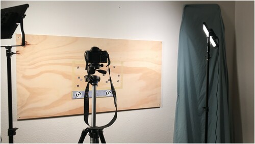
Table 1. Trials undertaken to determine the accuracy and precision of the workflow.

Trial		Epoch	Test board set-up	Light source
1	Control – Effect of registration technique	Epoch 1	Sixteen labels	LED panels
		Epoch 2	Sixteen labels	LED panels
2	Change detection – Effect of adding eight measured objects	Epoch 2	Sixteen labels	LED panels
		Epoch 3	Sixteen labels and eight objects	LED panels
3	Change detection – Effect of removing two measured labels	Epoch 3	Sixteen labels and eight objects	LED panels
		Epoch 4	Fourteen labels and eight objects	LED panels
4	Lighting test – Effect of moved LED panels	Epoch 4	Fourteen labels and eight objects	LED panels
		Epoch 5	Fourteen labels and eight objects	LEDs 20° towards the board
5	Lighting test – Effect of handheld flashes	Epoch 6	Fourteen labels and eight objects	Handheld flashes
		Epoch 7	Fourteen labels and eight objects	Handheld flashes
6	Lighting test – Effect of flashes on armature	Epoch 8	Fourteen labels and eight objects	Flashes on armature
		Epoch 9	Fourteen labels and eight objects	Flashes on armature
7	Lighting test – Effect of ring flash	Epoch 10	Fourteen labels and eight objects	Ring flash
		Epoch 11	Fourteen labels and eight objects	Ring flash
8	Lighting test – Effect of two different light sources	Epoch 7	Fourteen labels and eight objects	Handheld flashes
		Epoch 11	Fourteen labels and eight objects	Ring flash

Figure 5. The results of the control (Trial 1) comparing Epoch 1 and Epoch 2 show the change detected at each label point and its variation from zero. The small deviation from zero in the dataset shows that the epochs were closely aligned. © J. Paul Getty Trust

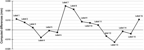
Table 2. Mean detected change and standard deviation on the DoD from the control and lighting trials.

Trial	Mean detected change	Standard deviation (σ)
Trial 1 – Control – LED panels	0.004 mm	±0.010 mm
Trial 4 – LED panels replaced 20° towards the board	0.004 mm	±0.019 mm
Trial 5 – Handheld flashes	0.003 mm	±0.015 mm
Trial 6 – Flashes on armature	0.007 mm	±0.014 mm
Trial 7 – Ring flash	−0.006 mm	±0.014 mm
Trial 8 – Ring flash vs handheld flashes	−0.002 mm	±0.031 mm

Figure 6. The orthophotos generated from the light sources created different shadow patterns on the test board. Only the ring flash resulted in no visible shadows on the orthophoto. © J. Paul Getty Trust

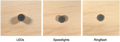
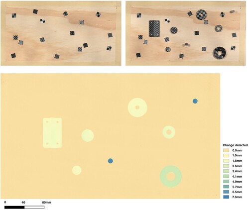
Figure 7. In Trial 2, the DEM of difference (DoD) (bottom) reflecting the detected change between Epoch 2 (top left) and Epoch 3 (top right) is shown as a heatmap. © J. Paul Getty Trust