Fast Robust Correlation for High-Dimensional Data

Figures & data

Table 1 Computation times (in seconds) of various correlation matrices as a function of the dimension d, for n = 1000 observations.

Dimension	MCD	OGK	SSCM	Spearman	Wrapping	Classic
10	0.319	0.022	0.004	0.002	0.003	0.001
50	6.222	0.426	0.009	0.009	0.012	0.002
100	24.76	2.089	0.031	0.019	0.027	0.008
500	1599	44.78	0.678	0.226	0.281	0.171
1000	–	166.7	3.107	0.774	0.836	0.685
5000	–	4389	129.1	17.11	17.39	16.81
10,000	–	–	568.9	68.24	68.78	67.27
20,000	–	–	2448	278.4	274.9	273.6

Fig. 1 Location influence functions at ρ = 0 for different transformations g.

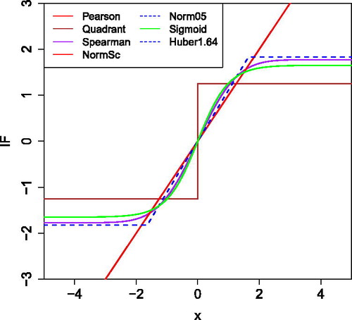
Fig. 2 The proposed transformation (22) with default constants b = 1.5 and c = 4.

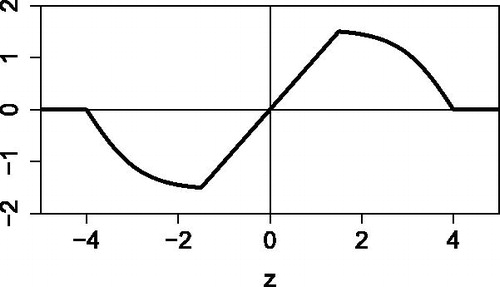
Table 2 Correlation measures based on transformations g with their breakdown value ${\epsilon }^{*}$, efficiency, gross-error sensitivity ${\gamma }^{*}$, rejection point ${\delta }^{*}$, and correlation between X and g(X).

${\text{cor}}_g$	${\epsilon }^{*}$(%)	eff (%)	${\gamma }^{*}$	${\delta }^{*}$	cor
Pearson	0	100	$\infty$	$\infty$	1
Quadrant	50	40.5	1.57	$\infty$	0.798
Spearman (SP)	20.6	91.2	3.14	$\infty$	0.977
Normal scores (NS)	12.4	100	$\infty$	$\infty$	1
Truncated NS, $\alpha =0.05$	16.3	95.0	3.34	$\infty$	0.987
Truncated NS, $\alpha =0.1$	20.7	88.9	2.57	$\infty$	0.971
Sigmoid	28.3	86.6	2.73	$\infty$	0.965
Huber, $b={\Phi }^{-1}(0.95)\approx 1.64$	23.5	95.0	3.34	$\infty$	0.987
Huber, $b={\Phi }^{-1}(0.9)\approx 1.28$	29.2	88.9	2.57	$\infty$	0.971
Wrapping, b = 1.5, c = 4	25.1	89.0	3.16	4.0	0.971
Wrapping, b = 1.3, c = 4	28.1	84.4	2.79	4.0	0.958

Fig. 3 Illustration of wrapping a standardized sample $\{z_1,\dots ,z_n\}$. Values in the interval $[-b,b]$ are left unchanged, whereas values outside $[-c,c]$ are zeroed. The intermediate values are “folded” inward so they still play a role.

Fig. 4 Bias and MSE of correlation measures based on transformation, for uncontaminated Gaussian data with sample size 100.

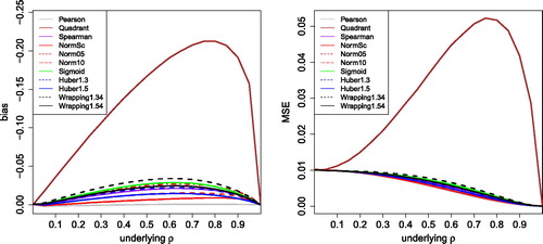
Fig. 5 MSE of the correlation measures in Figure 4 with 10% of outliers placed at k = 3 (left) and k = 5 (right).

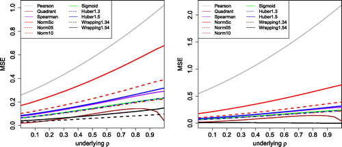
Fig. 6 Bias and MSE of other robust correlation measures, for uncontaminated Gaussian data with sample size 100.

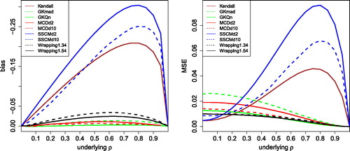
Fig. 7 MSE of the correlation measures in Figure 6 with 10% of outliers placed at k = 3 (left) and k = 5 (right).

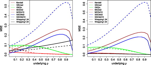
Fig. 8 Left panel: power of dCor (dashed black curve) and its robust version (blue curve) for bivariate X and Y with distribution t(1) and independence except for ${\mathit{X}}_1={\mathit{Y}}_1$ versus the sample size n. Right panel: power of dCor and its robust version for d-dimensional X and Y with distribution t(1) and n = 100, as a function of the dimension d.

Fig. 9 Prostate data: cellmap of the genes with the largest number of flagged cells.

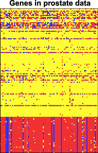
Fig. 10 Frames 60, 100, and 200 of the video data.

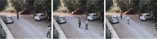
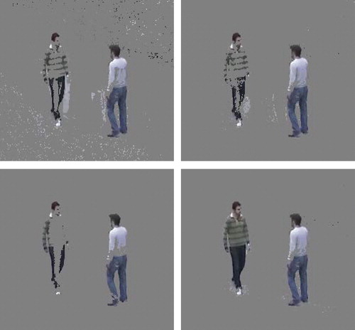
Fig. 11 First loading vector of the video data, for classical PCA (upper left), Spearman correlation (upper right), Huber’s ψ (lower left), and wrapping (lower right).

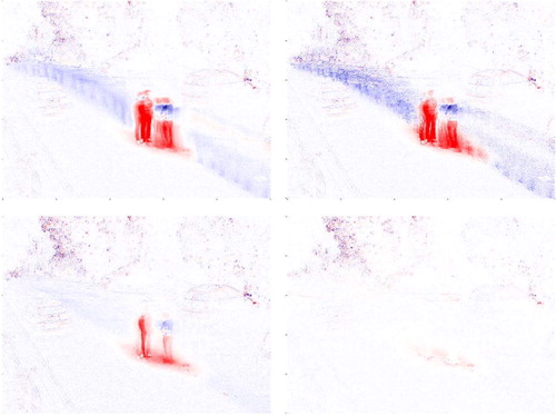
Fig. 12 Residuals of the video data, for classical PCA (upper left), Spearman correlation (upper right), Huber’s ψ (lower left), and wrapping (lower right).