Spectral Clustering on Spherical Coordinates Under the Degree-Corrected Stochastic Blockmodel

Figures & data

Fig. 1 Histogram of within-community degree distributions from three bipartite networks with size $439\times 60,635$, obtained from (a) a simulation of a SBM, (b) a simulation of a DCSBM, and (c) a real-world computer network (ICL2, see Section 6.2).

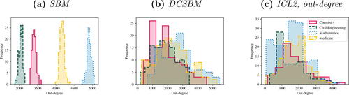
Fig. 2 Scatterplots of the two-dimensional ASE of a simulated DCSBM with (a) K = 4, and (b) K = 2. Figure 2(b) also highlights the true and estimated latent position for six nodes, with the corresponding 50%, 75%, and 90% contours from the ASE-CLT, and the estimated latent positions ${\widehat{\mathit{x}}}_{1,\mathcal{l}}$ for ${\mathit{x}}_1$ from simulated DCSBM adjacency matrices ${\mathbf{A}}_{\mathcal{l}},\mathcal{l}=1,\dots ,1000$.

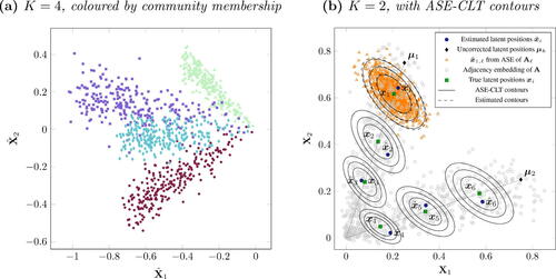
Fig. 3 Plots of ${\widehat{\mathit{x}}}_i,{\tilde{\mathit{x}}}_i={\widehat{\mathit{x}}}_i/\left|\right|{\widehat{\mathit{x}}}_i\left|\right|$ and ${\widehat{\theta }}_i=f_2({\widehat{\mathit{x}}}_i)$, obtained from the two-dimensional ASE of a simulated DCSBM. Joint (green) and community-specific (blue and red) marginal distributions with MLE Gaussian fit are also shown.

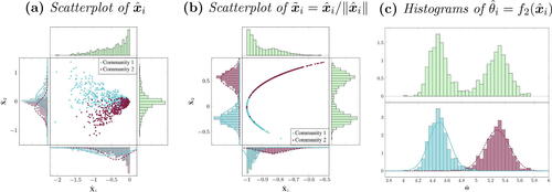
Fig. 4 Boxplots for $N=1000$ simulations of a degree-corrected stochastic blockmodel with $n=2000$ nodes, K = 3, equal number of nodes allocated to each group, and B described in (9), corrected by parameters ρ_i sampled from a $\text{Uniform}(0,1)$ distribution.

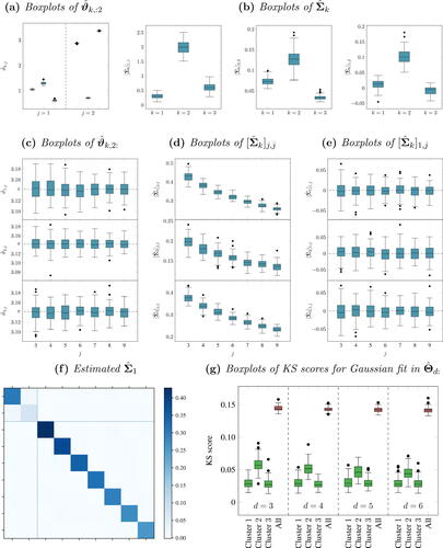
Table 1 Estimated performance for N = 250 simulated DCSBMs and bipartite DCScBMs.

(a) Undirected DCSBM
	K = 2			K = 3
	$\widehat{\mathbf{X}}$	$\tilde{\mathbf{X}}$	$\widehat{\mathbf{\Theta }}$	$\widehat{\mathbf{X}}$	$\tilde{\mathbf{X}}$	$\widehat{\mathbf{\Theta }}$
Proportion of correct d	0.788	0.796	0.972	0.740	0.736	0.748
Proportion of correct K	0.000	0.080	0.624	0.000	0.092	0.296
Average ARI	0.339	0.510	0.764	0.594	0.748	0.858
(b) Bipartite DCScBM
	K = 2			$K\prime =3$
	$\widehat{\mathbf{X}}$	$\tilde{\mathbf{X}}$	$\widehat{\mathbf{\Theta }}$	$\widehat{\mathbf{X}}\prime$	$\tilde{\mathbf{X}}\prime$	$\widehat{\mathbf{\Theta }}\prime$
Proportion of correct d	0.940	0.948	0.876	0.888	0.916	0.896
Proportion of correct K	0.000	0.056	0.580	0.000	0.096	0.540
Average ARI	0.374	0.564	0.885	0.490	0.572	0.715

Fig. 5 Estimated performance for N = 250 simulated DCSBMs and DCScBMs, for $n\in \{100,200,500,1000,2000\}$. For bipartite DCScBMs, $n\prime \in \{150,300,750,1500,3000\}$.

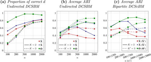
Fig. 6 Boxplots of differences in ARI for N = 250 simulated DCSBMs and DCScBM.

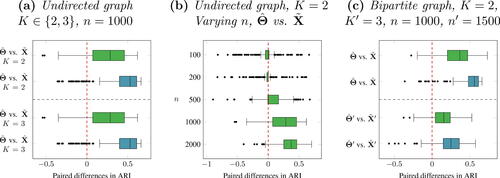
Table 2 Summary statistics for the Imperial College London computer networks.

Name	$\left|V\right|$	$|V\prime |$	$\left|E\right|$	K	ZG3	ZG4
ICL1	628	54,111	668,155	3	24	52
ICL2	439	60,635	717,912	4	24	53
ICL3	1011	84,664	1,470,074	5	27	51

Fig. 7 ICL2: scatterplot of the leading two dimensions for $\widehat{\mathbf{X}}$, $\tilde{\mathbf{X}}$ and $\widehat{\mathbf{\Theta }}$.

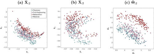
Table 3 Estimates of (d, K) and ARIs for the embeddings $\widehat{\mathbf{X}},\tilde{\mathbf{X}}$ and $\widehat{\mathbf{\Theta }}$ for $m\in \{30,50\}$ and alternative methodologies.

(a) Estimated (d, K)
	m = 30			m = 50
	$\widehat{\mathbf{X}}$	$\tilde{\mathbf{X}}$	$\widehat{\mathbf{\Theta }}$	$\widehat{\mathbf{X}}$	$\tilde{\mathbf{X}}$	$\widehat{\mathbf{\Theta }}$
ICL1	(26, 6)	(11, 6)	(11, 4)	(22, 5)	(11, 6)	(11, 4)
ICL2	(28, 5)	(8, 7)	(15, 4)	(29, 4)	(8, 7)	(15, 4)
ICL3	(24, 10)	(17, 5)	(15, 5)	(25, 6)	(13, 6)	(16, 5)
(b) ARIs for the estimated clustering
	m = 30			m = 50			Alternative methods
	$\widehat{\mathbf{X}}$	$\tilde{\mathbf{X}}$	$\widehat{\mathbf{\Theta }}$	$\widehat{\mathbf{X}}$	$\tilde{\mathbf{X}}$	$\widehat{\mathbf{\Theta }}$	Louvain	Paris	HLouvain
ICL1	0.259	0.324	0.418	0.262	0.317	0.418	0.107	0.082	0.152
ICL2	0.441	0.736	0.938	0.359	0.743	0.938	0.488	0.560	0.602
ICL3	0.246	0.342	0.409	0.269	0.265	0.364	0.079	0.032	0.157