Deep Gaussian Process Emulation using Stochastic Imputation

Figures & data

Fig. 1 The hierarchy of GPs that represents a feed-forward system of two computer models.

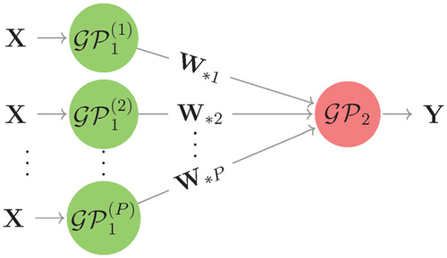
Fig. 2 The generic DGP hierarchy considered to illustrate the Stochastic Imputation (SI).

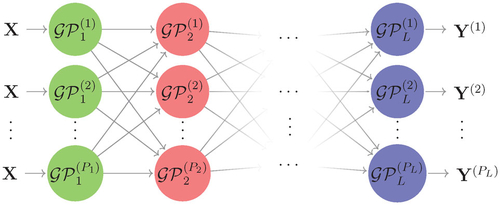
Fig. 3 The two-layered elementary DGP model that is targeted by ESS-within-Gibbs to sample a realization of output ${\mathbf{W}}_l^{(p)}$ from $\mathcal{G}{\mathcal{P}}_l^{(p)}$ given all other latent variables.

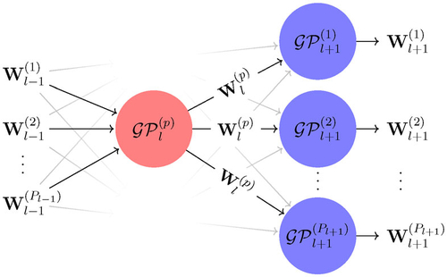
Fig. 4 DGP emulators of the step function (the solid line) trained by different inference methods. The dashed line is the mean prediction; the shaded area is the predictive interval (i.e., two predictive standard deviations above and below the predictive mean); the filled circles are training points.

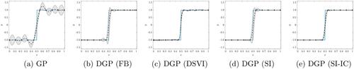
Fig. 5 Predictive standard deviations of GP and DGP emulators over the input domain. The shaded area in (b) to (e) represents the interval between the 5th and 95th percentiles (with the dash line highlighting the 50th percentile) of 100 predictive standard deviations produced by the corresponding 100 repeatedly trained DGPs; 30 out of 100 predictive standard deviations are randomly selected and drawn as the solid lines in (b) to (e). The underlying true step function and training input locations (shown as filled circles) are projected into all sub-figures.

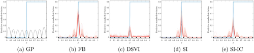
Fig. 6 Comparison of FB, DSVI, SI, and SI-IC across 100 repeatedly trained DGP emulators and the corresponding implementation packages’ computation time. (a): Violin plots of Normalized Root Mean Squared Error of Predictions (NRMSEPs). The dash-dot line represents the trained conventional GP. (b): Average computation time (including training and prediction) per trial.

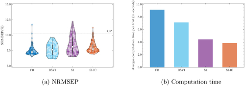
Fig. 7 Contour plots of a slice of Vega, Delta and Gamma produced by (10) over $(S_t,K)\in {[10,200]}^2$ when τ = 1.

Fig. 8 Three different DGP formations considered to build the emulator of Vega.

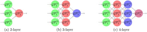
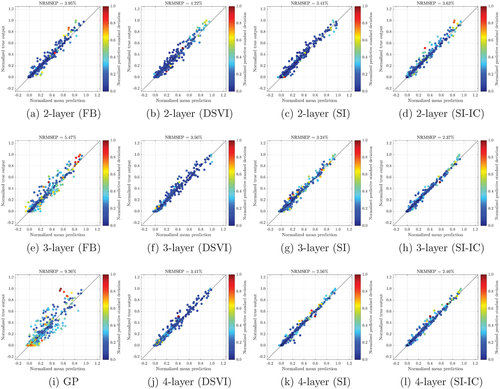
Fig. 9 Comparison of FB, DSVI, SI, and SI-IC for 40 repeatedly trained DGP emulators (i.e., 40 inference trials) of Vega (${\mathcal{V}}_t$) from the Heston model. FB is not implemented for the 4-layer formation because deepgp only allows DGPs up to three layers. The dash-dot line represents the NRMSEP of a trained conventional GP emulator.

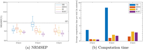
Fig. 10 Plots of numerical solutions of Vega (${\mathcal{V}}_t$) (normalized by their max and min values) from the Heston model at 500 testing positions versus the mean predictions (normalized by the max and min values of numerical solutions of Vega), along with predictive standard deviations (normalized by their max and min values), made by the best emulator (with the lowest NRMSEP out of 40 inference trials) produced by FB, DSVI, SI, and SI-IC. GP represents a conventional GP emulator.