Active sampling: A machine-learning-assisted framework for finite population inference with optimal subsamples

Figures & data

Figure 1 A: Simulated impact speed reduction with an automatic emergency braking system (AEB) compared to a baseline manual driving scenario (without AEB) in a computer experiment of a rear-end collision generation. In the bottom right corner, no crash was generated in the baseline scenario; such instances are non-informative with regards to safety benefit evaluation. B: Corresponding optimal active sampling scheme. Active sampling oversamples instances in regions where there is a high probability of generating a collision in the baseline scenario (attempting to generate only informative instances) and with a large predicted deviation from the average. These instances will be influential for estimating the safety benefit of the AEB system.

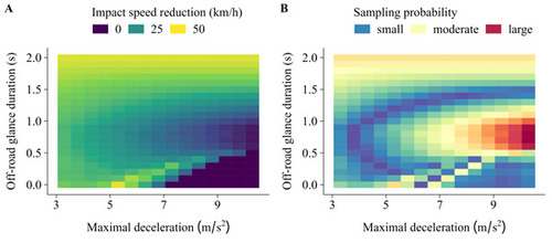
Figure 2 Examples of three synthetic datasets with varying degree of non-linearity. Data were generated according to a Gaussian process, using a Gaussian kernel with bandwidth σ.

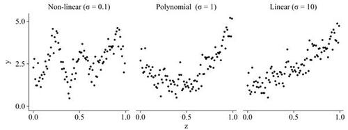
Figure 3 Performance of active sampling using a linear surrogate model (LM) or generalized additive surrogate model (GAM) compared to simple random sampling, ratio estimator, control variates, and importance sampling for estimating a finite population mean in a strictly positive scenario (all $y_i>0$) using a linear estimator ( $h(u)=u/N$) and batch size n_k = 10. Results are shown for 12 different scenarios with varying signal-to-noise ratio (R²) and varying degree of non-linearity (σ) (cf. Figure 2). Shaded regions are 95% confidence intervals for the root mean squared error of the estimator (eRMSE) based on 500 repeated subsampling experiments. Asterisks show the smallest sample sizes for which there were persistent significant improvements (p <.05) with active sampling compared to simple random sampling.

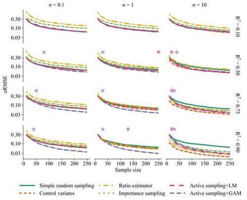
Figure 4 Empirical coverage rates of 95% confidence intervals for the mean impact speed reduction (A) and crash avoidance rate (B) using active sampling. The lines show the coverage rates with three different methods for variance estimation in 500 repeated subsampling experiments. A batch size of n_k = 10 observations per iteration was used.

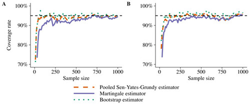
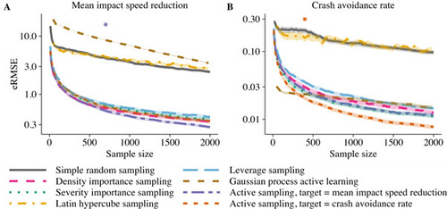
Figure 5 Root mean squared error (eRMSE) for estimating the mean impact speed reduction (A) and crash avoidance rate (B). The lines show the performance using simple random sampling, importance sampling, Latin hypercube sampling, leverage sampling, Gaussian process active learning, and active sampling optimized for the estimation of the mean impact speed reduction and crash avoidance rate. Shaded regions represent 95% confidence intervals for the eRMSE based on 500 repeated subsampling experiments. Asterisks show the smallest sample sizes for which there were persistent significant improvements (p <.05) with active sampling compared to the best performing benchmark method.