Unsteady-state brush theory

Figures & data

Figure 1. Tyre schematic for the pure longitudinal problem ($V_y\left(t\right)={\omega }_z\left(t\right)=0$). The bristles and the tyre carcass (modelled as a linear spring) are drawn in red. The generalised forces acting on the tyre-wheel system are represented in blue. The speeds are finally given in green. The dot notation stands for total derivative with respect to time. The local variable $\xi =x_L(y,{\mathit{\rho }}_{x_L}(t\left)\right)-x$ is referred as the distance from the leading edge.

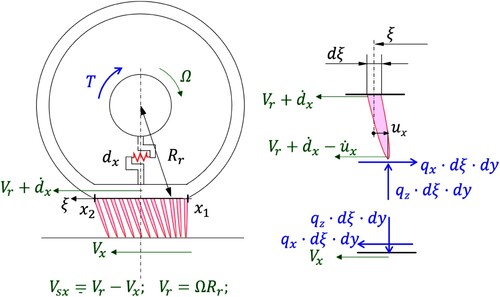
Figure 2. Time trend for the shear stresses $q_y(\xi ,\varsigma )$ in the contact patch for case I. The three figures refer to different values of the nondimensional travelled distance $\overline{\varsigma }$. Since the trend for the solution $u_y^{+}\left(\varsigma \right)$ in the adhesion region is constant, the steady-state condition is reached when $\overline{\varsigma }=1$, or, equivalently, when the travelled distance equals the contact length.

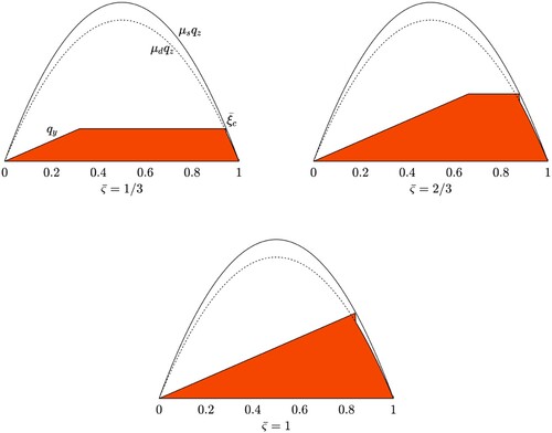
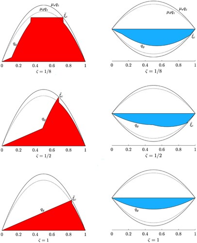
Figure 3. Time trend for the shear stresses $q_y(\xi ,\varsigma )$ in the contact patch for case II. The three figures refer to different values of the nondimensional travelled distance $\overline{\varsigma }$. Since the trend for the solution $u_y^{+}\left(\varsigma \right)$ in the adhesion region is constant, the steady-state condition is reached when $\overline{\varsigma }=\frac{3}{4}\left({\mu }_s{F}_z/C_{y\alpha }|{\sigma }_y|\right)$, or, equivalently, when the travelled distance equals the value ${\varsigma }^{\ast }$.

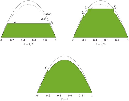
Figure 4. Time trend for the shear stresses $q_y(\xi ,\varsigma )$ in the contact patch for case III. The three figures refer to different values of the nondimensional travelled distance $\overline{\varsigma }$. Since the trend for the solution $u_y^{+}\left(\varsigma \right)$ in the adhesion region is constant, the steady-state condition is reached when $\overline{\varsigma }=\frac{3}{4}\left({\mu }_s{F}_z/C_{y\alpha }|{\sigma }_y|\right)$, or, equivalently, when the travelled distance equals the value ${\varsigma }^{\ast }$.

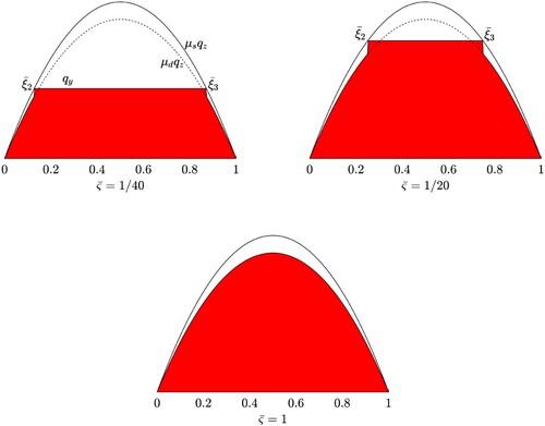
Figure 5. Time trend for the shear stresses $q_y(\xi ,\varsigma )$ in the contact patch due to pure camber. The three figures refer to different values of the nondimensional travelled distance $\overline{\varsigma }$. Since the trends for the solutions $u_y^{-}\left(\xi \right)$ and $u_y^{+}(\xi ,\varsigma )$ in the adhesion region are parabolic and linear, respectively, the steady-state condition is only reached when $\overline{\varsigma }$ = 1, or, equivalently, when the travelled distance equals the contact length.

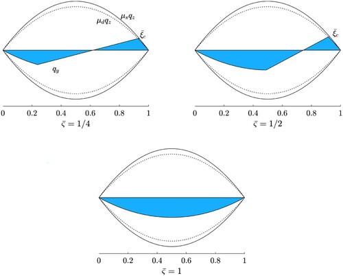
Figure 6. Time trend for the shear stresses $q_y(\xi ,\varsigma )$ in the contact patch due to pure lateral interaction and pure camber, respectively, starting from nonzero initial conditions $u_y^0\ne 0$. The figures refer to different values of the nondimensional travelled distance $\overline{\varsigma }$. The initial condition for the pure lateral case (left-hand side panel) corresponds to a transient trend for the deformation of the bristles due to an initial slip value ${\sigma }_y^0>{\sigma }_y^{crit}$. The transient solution for the camber (right-hand side panel) refers to a case in which the initial spin value ${\gamma }^0$ has the same sign as the current one. The initial condition corresponds to a steady-state trend of the bristle displacement.

Table

Forces and Moments	Unit	Description
${\mathit{F}}_t$	N	Planar forces vector
${\mathit{F}}_t^{\star }$	N	Augmented planar forces vector
$F_{y\alpha }$	N	Lateral force due to lateral slip
$F_{y\gamma }$	N	Lateral force due to camber
$F_z$	N	Vertical force applied at the rim centre
$M_z$	$\mathrm{N}\cdot \mathrm{m}$	Self-aligning torque
${\mathit{q}}_t$	$\mathrm{N}/{\mathrm{m}}^2$	Planar shear stresses vector
$q_x$	$\mathrm{N}/{\mathrm{m}}^2$	Longitudinal shear stress
$q_y$	$\mathrm{N}/{\mathrm{m}}^2$	Lateral shear stress
$q_z$	$\mathrm{N}/{\mathrm{m}}^2$	Vertical pressure
Displacements	Unit	Description
${\mathit{S}}_s^{\star }$	m, rad	Augmented sliding displacements vector
$S_{sy}$	m	Lateral sliding displacement
$\mathit{d}$	m	Tyre carcass displacement vector
${\mathit{d}}^{\star }$	m	Augmented carcass displacement vector
$d_x$	m	Longitudinal displacement of the tyre carcass
$d_y$	m	Lateral displacement of the tyre carcass
${\mathit{u}}_t$	m	Bristle deflection vector
${\mathit{u}}_t^{-}$	m	Bristle deflection vector for $\xi <\varsigma$
${\mathit{u}}_t^{+}$	m	Bristle deflection vector $\xi \ge \varsigma$
${\overline{\mathit{u}}}_t$	–	Nondimensional bristle deflection vector
${\mathit{u}}_t^a$	m	Bristle deflection vector in the adhesion region
$u_x$	m	Bristle longitudinal deflection
$u_x^{-}$	m	Bristle longitudinal deflection for $\xi <\varsigma$
$u_x^{+}$	m	Bristle longitudinal deflection for $\xi \ge \varsigma$
${\overline{u}}_x$	–	Nondimensional bristle longitudinal deflection
$u_y$	m	Bristle lateral deflection
$u_y^{-}$	m	Bristle lateral deflection for $\xi <\varsigma$
$u_y^{+}$	m	Bristle lateral deflection for $\xi \ge \varsigma$
${\overline{u}}_y$	–	Nondimensional bristle lateral deflection
$\mathit{x}$	m	Planar coordinate vector
x	m	Longitudinal coordinate
y	m	Lateral coordinate
η	m	Parametric lateral coordinate
ξ	m	Distance from the entrance
$\overline{\xi }$	–	Nondimensional distance from the entrance
${\xi }_c$	m	Breakaway point position
ς	m	Travelled distance
$\overline{\varsigma }$	–	Nondimensional travelled distance
Speeds	Unit	Description
$\mathit{V}$	$\mathrm{m}/\mathrm{s}$	Speed vector
$V_r$	$\mathrm{m}/\mathrm{s}$	Tyre rolling speed
$V_x$	$\mathrm{m}/\mathrm{s}$	Longitudinal speed of the rim
$V_y$	$\mathrm{m}/\mathrm{s}$	Lateral speed of the rim
${\mathit{V}}_s$	$\mathrm{m}/\mathrm{s}$	Sliding speed vector
${\mathit{V}}_s^{\star }$	$\mathrm{m}/\mathrm{s}$	Augmented sliding speed vector
$V_{sx}$	$\mathrm{m}/\mathrm{s}$	Longitudinal sliding speed
$V_{sy}$	$\mathrm{m}/\mathrm{s}$	Lateral sliding speed
${\mathit{v}}_s$	$\mathrm{m}/\mathrm{s}$	Micro-sliding speed vector
${\mathit{v}}_s^{\mathrm{\prime }}$	$\mathrm{m}/\mathrm{s}$	Approximated micro-sliding speed vector
$v_{sx}$	$\mathrm{m}/\mathrm{s}$	Micro-sliding longitudinal speed
$v_{sy}$	$\mathrm{m}/\mathrm{s}$	Micro-sliding lateral speed
$v_{sx}^{\mathrm{\prime }}$	$\mathrm{m}/\mathrm{s}$	Approximated micro-sliding longitudinal speed
$v_{sy}^{\mathrm{\prime }}$	$\mathrm{m}/\mathrm{s}$	Approximated micro-sliding lateral speed
$\dot{\psi }$	$\mathrm{r}\mathrm{a}\mathrm{d}/\mathrm{s}$	Steering speed
Ω	$\mathrm{r}\mathrm{a}\mathrm{d}/\mathrm{s}$	Angular speed of the rim
${\omega }_z$	$\mathrm{r}\mathrm{a}\mathrm{d}/\mathrm{s}$	Angular speed around the z axis
Slip Parameters	Unit	Description
φ	–	Rotational slip or spin parameter
$\mathit{\sigma }$	–	Translational slip vector
${\mathit{\sigma }}^{\star }$	–	Augmented translational slip vector
${\sigma }_x$	–	Longitudinal slip
${\sigma }_y$	–	Lateral slip
Geometrical Parameters	Unit	Description
$R_r$	m	Rolling radius
l	m	Contact patch length
w	m	Contact patch width
$x_L$	m	Leading edge position
$x_T$	m	Trailing edge position
γ	rad	Camber angle
Stiffnesses and Compliances	Unit	Description
${\mathbf{C}}^{\mathrm{\prime }}$	$\mathrm{N}/\mathrm{m}$	Carcass stiffness matrix
$C_x^{\mathrm{\prime }}$	$\mathrm{N}/\mathrm{m}$	Carcass longitudinal stiffness
$C_y^{\mathrm{\prime }}$	$\mathrm{N}/\mathrm{m}$	Carcass lateral stiffness
$C_{y\alpha }$	N	Cornering stiffness
$C_{y\gamma }$	N	Camber stiffness
${\mathbf{k}}_t$	$\mathrm{N}/{\mathrm{m}}^3$	Matrix of the bristle tangential stiffnesses
$k_x$	$\mathrm{N}/{\mathrm{m}}^3$	Bristle longitudinal stiffness
$k_y$	$\mathrm{N}/{\mathrm{m}}^3$	Bristle lateral stiffness
$\mathbf{\Gamma }$	$\mathrm{m}/\mathrm{N}$	Carcass compliance matrix
Friction Parameters	Unit	Description
${\mu }_d$	–	Sliding friction coefficient
${\mu }_s$	–	Sticking friction coefficient
Functions and Operators	Unit	Description
${\mathbf{\Sigma }}_1(\bullet ),{\mathbf{\Sigma }}_2(\bullet )$	–	Sigma functions