Brush tyre models for large camber angles and steering speeds

Figures & data

Figure 1. Tyre-road schematics in the Oxz and Oyz planes (left and right-hand side figures, respectively). The geometric parameters are drawn in black, the kinematic quantities in green, the generalised forces in blue and the elastic displacements in red. The dimension and the deformation of the bristles have been exaggerated to facilitate the visualisation.

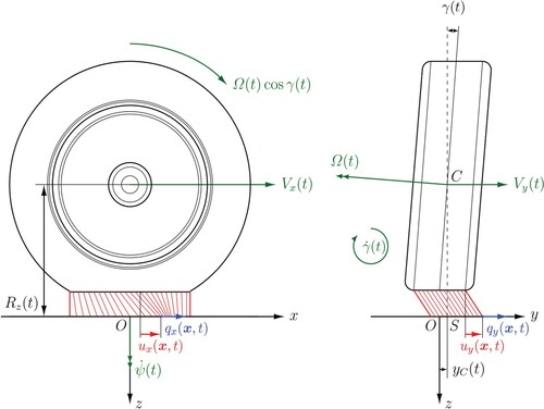
Figure 2. Subdomains ${\mathcal{P}}_1$, ${\mathcal{P}}_2$ and ${\mathcal{P}}_3$ of the contact patch $\mathcal{P}$ (represented by the rectangles) for different values of the camber angle $\gamma =10$, 30, 50 and ${70}^{\circ }$, respectively. The larger green area corresponds to the domain ${\mathcal{P}}_1$, whilst the red and blue one to ${\mathcal{P}}_2$ and ${\mathcal{P}}_3$. The arrows represent the velocity field ${\mathit{v}}_{\mathit{t}}\left(\mathit{x}\right)$ and are always tangent to the trajectories of the bristles, which coincide with the characteristics lines given by (41a(41a) $\begin{array}{rl}{c}_1& =(x-x_C{)}^2+{\left(y-y_C-\frac{R_{\text{r}}}{\sin \gamma }\right)}^2,\end{array}$(41a) ). The length and the width of the contact patch are l = 0.1 and w = 0.07 (m). (a) Domains ${\mathcal{P}}_1$, ${\mathcal{P}}_2$ and ${\mathcal{P}}_3$ for a camber angle of $\gamma ={10}^{\circ }$. (b) Domains ${\mathcal{P}}_1$, ${\mathcal{P}}_2$ and ${\mathcal{P}}_3$ for a camber angle of $\gamma ={30}^{\circ }$. (c) Domains ${\mathcal{P}}_1$, ${\mathcal{P}}_2$ and ${\mathcal{P}}_3$ for a camber angle of $\gamma ={50}^{\circ }$. (d) Domains ${\mathcal{P}}_1$, ${\mathcal{P}}_2$ and ${\mathcal{P}}_3$ for a camber angle of $\gamma ={70}^{\circ }$.

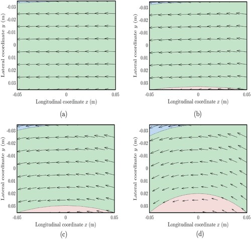
Figure 3. Steady-state and transient domains for each region of $\mathcal{P}$ for a constant value of the camber angle $\gamma ={70}^{\circ }$ and different travelled distances $\overline{s}=1/16$, 1/8, 1/4 and 1/2. The green, red and blue solid lines represent the interface between the steady-state and transient solution in the domains ${\mathcal{P}}_1$, ${\mathcal{P}}_2$ and ${\mathcal{P}}_3$, respectively. More specifically, the steady-state regions correspond to the right portion of the green and red areas for ${\mathcal{P}}_1$ and ${\mathcal{P}}_2$, and to the upper part of the blue domain for ${\mathcal{P}}_3$. It can be noted that steady-state conditions are reached in the region ${\mathcal{P}}_3$ relatively faster (the transient extinguishes in the blue area already for $\overline{s}=1/2$). The length and the width of the contact patch are l = 0.1 and w = 0.07 (m). (a) Steady-state and transient domains for each region of $\mathcal{P}$ for $\overline{s}=1/16$. (b) Steady-state and transient domains for each region of $\mathcal{P}$ for $\overline{s}=1/8$. (c) Steady-state and transient domains for each region of $\mathcal{P}$ for $\overline{s}=1/4$. (d) Steady-state and transient domains for each region of $\mathcal{P}$ for $\overline{s}=1/2$.

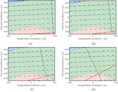
Figure 4. Steady-state and transient domains for each region of $\mathcal{P}$ for a constant value of the camber angle $\gamma ={70}^{\circ }$ and different travelled distances $\overline{s}=1/8$ and 1/2. The functions ${\mathrm{\Sigma }}_1$ ${\mathrm{\Sigma }}_2$ and ${\mathrm{\Sigma }}_3$ correspond to the green, red and blue curve, respectively, and represent the interface between the steady-state and blacktransient blacksolution in the domains ${\mathcal{P}}_1$, ${\mathcal{P}}_2$ and ${\mathcal{P}}_3$. It can be seen that they rotate tangentially to the circumferences ${\mathcal{C}}_0$, ${\mathcal{C}}_1$ and ${\mathcal{C}}_3$. (a) Steady-state and transient subdomains of the contact patch $\mathcal{P}$ corresponding to a normalised travelled distance of $\overline{s}=1/8$. (b) Steady-state and transient subdomains of the contact patch $\mathcal{P}$ corresponding to a normalised travelled distance of $\overline{s}=1/2$.

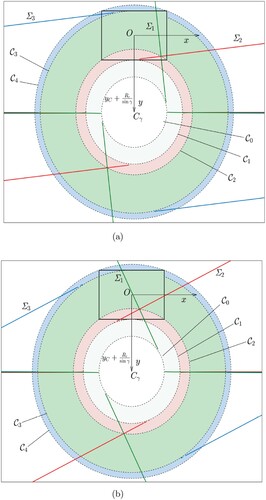
Figure 5. Transient trend of the total shear stress $q_{\mathit{t}}(\mathit{x},s)$ ($k_x=8\cdot {10}^7$ $\text{N}{\text{m}}^{-3}$, $k_y=0.7k_x$) predicted by the different models for two values of the normalised travelled distance $\overline{s}=1/2$ (left-hand side subplot) and $\overline{s}=2$ (right-hand side subplot). The figures refer to the following values of the kinematic parameters: ${\sigma }_x={\sigma }_y=0.1$, $\phi =1$, ${ϵ}_{\psi }=0.5$. (a) Total shear stress $q_{\mathit{t}}(\mathit{x},s)$ predicted using the 1DCM. The left and right-hand side subplots refer to a value of the normalised travelled distance of $\overline{s}=1/2$ and 2, respectively. (b) Total shear stress $q_{\mathit{t}}(\mathit{x},s)$ predicted using the 2DM. The left and right-hand side subplots refer to a value of the normalised travelled distance of $\overline{s}=1/2$ and 2, respectively. (c) Total shear stress $q_{\mathit{t}}(\mathit{x},s)$ predicted using the 2DCM. The left and right-hand side subplots refer to a value of the normalised travelled distance of $\overline{s}=1/2$ and 2 respectively.

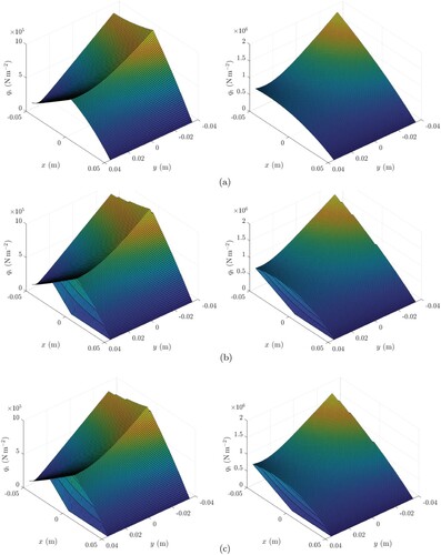
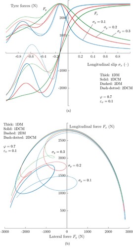
Figure 6. Tyre characteristics versus the longitudinal slip ${\sigma }_x$ for different discrete values of the lateral slip ${\sigma }_y$ and steering ratio ${ϵ}_{\psi }$. (a) Longitudinal and lateral tyre characteristics versus the longitudinal slip ${\sigma }_x$ for different values of the lateral slip ${\sigma }_y$ and steering ratio ${ϵ}_{\psi }=0.1$. (b) Longitudinal and lateral tyre characteristics versus the longitudinal slip ${\sigma }_x$ for different values of the lateral slip ${\sigma }_y$ and steering ratio ${ϵ}_{\psi }=0.9$.

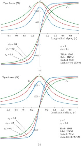
Figure 7. Self-aligning moment versus the longitudinal slip ${\sigma }_x$ for different discrete values of the lateral slip ${\sigma }_y$ and steering ratio ${ϵ}_{\psi }$. It can be noted that, for small values of the steering ratio, the 2DM and 2DCM both succeed in estimating the true trend of the self-aligning moment, where the other theories fail; conversely, for larger values of ${ϵ}_{\psi }$, the trend is better predicted by the 1DCM and 2DCM. (a) Self-aligning moment versus the longitudinal slip ${\sigma }_x$ for different values of the lateral slip ${\sigma }_y$ and steering ratio ${ϵ}_{\psi }=0.1$. (b) Self-aligning moment versus the longitudinal slip ${\sigma }_x$ for different values of the lateral slip ${\sigma }_y$ and steering ratio ${ϵ}_{\psi }=0.9$.

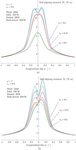
Figure 8. Friction ellipses for different discrete values of the lateral slip ${\sigma }_y$ and steering ratio ${ϵ}_{\psi }$. It can be noted that, for small values of the steering ratio, the 2DM and 2DCM both succeed in estimating the true trend of the self-aligning moment, where the other theories fail; conversely, for larger values of ${ϵ}_{\psi }$, the trend is better predicted by the 1DCM and 2DCM. (a) Friction ellipse for different values of the lateral slip ${\sigma }_y$ and steering ratio ${ϵ}_{\psi }=0.1$. (b) Friction ellipse for different values of the lateral slip ${\sigma }_y$ and steering ratio ${ϵ}_{\psi }=0.9$.

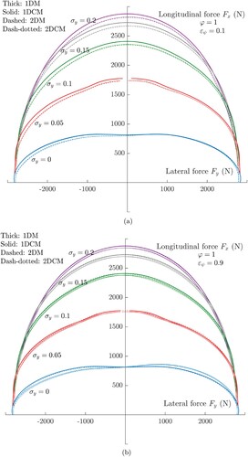
Figure 9. $F_y-M_z$ diagram for different discrete values of the lateral slip ${\sigma }_y$ and steering ratio ${ϵ}_{\psi }$. It can be noted that, for small values of the steering ratio, the 2DM and 2DCM both succeed in estimating the true trend of the self-aligning moment, where the other theories fail; conversely, for larger values of ${ϵ}_{\psi }$, the trend is better predicted by the 1DCM and 2DCM. (a) $F_y-M_z$ diagram for different values of the lateral slip ${\sigma }_y$ and steering ratio ${ϵ}_{\psi }=0.1$. (b) $F_y-M_z$ diagram for different values of the lateral slip ${\sigma }_y$ and steering ratio ${ϵ}_{\psi }=0.1$.

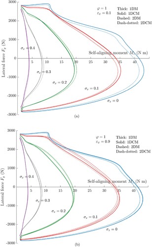
Figure 10. Tyre forces and friction ellipse for an heavily cambered tyre ($\gamma \approx {40}^{\circ }$). When the tyre experiences high level of cambering, the results predicted by the two-dimensional theories exhibit appreciable differences with the ones found by means of the 1DM and 1DCM. (a) Longitudinal and lateral tyre characteristics versus the longitudinal slip ${\sigma }_x$ for different values of the lateral slip ${\sigma }_y$ and steering ratio ${ϵ}_{\psi }=0.1$ and 0.9, respectively. The tyre rolling radius and the lateral coordinate of the wheel hub centre modelled as a function of the camber angle γ. (b) Friction ellipse for different values of the lateral slip ${\sigma }_y$ and steering ratio ${ϵ}_{\psi }=0.1$. The tyre rolling radius and the lateral coordinate of the wheel hub centre modelled as a function of the camber angle γ.

Table

Forces and Moments	Unit	Description
${\mathit{q}}_{\mathit{t}}$	${\text{N m}}^{-2}$	Tangential shear stress vector
$q_{\mathit{t}}$	${\text{N m}}^{-2}$	Total tangential shear stress
${\mathit{F}}_{\mathit{t}}$	N	Tangential force vector
$F_x$	N	Longitudinal tyre force
$F_y$	N	Longitudinal tyre force
$F_z$	N	Vertical force acting on the tyre
$M_z$	$\text{N}\text{m }$	Self-aligning moment
Displacements	Unit	Description
${\mathit{u}}_{\mathit{t}}$	m	Bristle tangential deflection vector
${\mathit{u}}_{\mathit{t}}^{-}$	m	Steady-state tangential displacement vector of the bristle
${\mathit{u}}_{\mathit{t}}^{+}$	m	Transient tangential displacement vector of the bristle
${\mathit{u}}_{\mathit{t}0}$	m	Initial tangential displacement vector of the bristle (IC)
$u_x^{-}$	m	Steady-state longitudinal deflection
$u_x^{+}$	m	Transient longitudinal deflection
$u_{x0}$	m	Initial longitudinal deflection (IC)
$u_y^{-}$	m	Steady-state lateral deflection
$u_y^{+}$	m	Transient lateral deflection
$u_{y0}$	m	Initial lateral deflection (IC)
s	m	Travelled distance
$\mathit{x}$	m	Planar coordinate vector
${\mathit{x}}_0$	m	Initial data vector (ID)
x	m	Longitudinal coordinate
$x_0$	m	Initial lateral datum (ID)
y	m	Lateral coordinate
$y_0$	m	Initial lateral datum (ID)
η	m	Alternative lateral coordinate
ξ	m	Alternative longitudinal coordinate or distance from the entrance
ζ	m	Alternative vertical coordinate
Speeds	Unit	Description
$\mathit{v}$	$\text{m}{\text{s}}^{-1}$	Three-dimensional velocity field
${\mathit{v}}_{\mathit{t}}$	$\text{m}{\text{s}}^{-1}$	Tangential velocity field
$v_x$	$\text{m}{\text{s}}^{-1}$	Longitudinal component of the velocity field
$v_y$	$\text{m}{\text{s}}^{-1}$	Lateral component of the velocity field
${\mathit{v}}_{\text{s}\mathit{t}}$	$\text{m}{\text{s}}^{-1}$	Micro-sliding tangential speed vector
$v_{\text{s}x}$	$\text{m}{\text{s}}^{-1}$	Micro-sliding longitudinal speed
$v_{\text{s}y}$	$\text{m}{\text{s}}^{-1}$	Micro-sliding lateral speed
$Vr$	$\text{m}{\text{s}}^{-1}$	Tyre rolling speed
$V_x$	$\text{m}{\text{s}}^{-1}$	Longitudinal speed of the wheel hub
$V_y$	$\text{m}{\text{s}}^{-1}$	Lateral speed of the wheel hub
${\mathit{V}}_{\text{s}\mathit{t}}$	$\text{m}{\text{s}}^{-1}$	Tangential macro-sliding speed vector
$V_{\text{s}x}$	$\text{m}{\text{s}}^{-1}$	Longitudinal macro-sliding speed
$V_{\text{s}y}$	$\text{m}{\text{s}}^{-1}$	Lateral macro-sliding speed
$\dot{\psi }$	$\text{rad}{\text{s}}^{-1}$	Steering speed
${\omega }_z$	$\text{rad}{\text{s}}^{-1}$	Angular speed around the z axis
Ω	$\text{rad}{\text{s}}^{-1}$	Angular speed of the rim
Slip	Unit	Description
Parameters
${ϵ}_{\gamma }$	–	Camber ratio
${ϵ}_{\psi }$	–	Steering ratio
$\mathit{\sigma }$	–	Translational slip vector
${\sigma }_x$	–	Longitudinal slip
${\sigma }_y$	–	Lateral slip
φ	–	Rotational slip or spin parameter
Geometrical	Unit	Description
Parameters
l	m	Contact patch length
w	m	Contact patch width
${\mathit{x}}_C$	m	Wheel hub centre coordinate vector
$x_C$	m	Wheel hub centre longitudinal coordinate
$x_{\mathcal{L}}$	m	Leading edge position
$y_C$	m	Wheel hub centre lateral coordinate
γ	rad	Camber angle
$R_0$	m	Radius of the circumference ${\mathcal{C}}_0$
$R_1$	m	Radius of the circumference ${\mathcal{C}}_1$
$R_2$	m	Radius of the circumference ${\mathcal{C}}_2$
$R_3$	m	Radius of the circumference ${\mathcal{C}}_3$
$R_4$	m	Radius of the circumference ${\mathcal{C}}_4$
$R_5$	m	Radius of the circumference ${\mathcal{C}}_5$
$Rr$	m	Rolling radius
$R_z$	m	Vertical radius
$R_{\delta }$	m	Tyre deformed radius
Stiffnesses	Unit	Description
and Compliances
$k_x$	$\text{N}{\text{m}}^{-3}$	Bristle longitudinal stiffness
$k_y$	$\text{N}{\text{m}}^{-3}$	Bristle lateral stiffness
${\mathbf{K}}_{\mathit{t}}$	$\text{N}{\text{m}}^{-3}$	Matrix of the bristle tangential stiffnesses
Friction	Unit	Description
Parameters
$\mu d$	–	Sliding friction coefficient
$\mu s$	–	Sticking friction coefficient
Functions and Operators	Unit	Description
${\text{D}}_{\mathit{t}}$	${\text{s}}^{-1}$	Tangential partial differential operator
${\mathrm{\nabla }}_{\mathit{t}}$	${\text{m}}^{-1}$	Tangential gradient
${\mathrm{\Phi }}_X(\cdot )$	${\text{m}}^3{\text{s}}^{-1}$	Flux through X
Γ	${\text{m}}^2$	Gamma function
Ξ	–	Xi function
${\mathrm{\Sigma }}_1,{\mathrm{\Sigma }}_2,{\mathrm{\Sigma }}_3$	m	Sigma functions
${\mathrm{\Phi }}_{1x},{\mathrm{\Phi }}_{2x},{\mathrm{\Phi }}_{3x}$	m	Phi functions for the longitudinal deflection
${\mathrm{\Phi }}_{1y},{\mathrm{\Phi }}_{2y},{\mathrm{\Phi }}_{3y}$	m	Phi functions for the lateral deflection
${\mathrm{\Psi }}_{1x},{\mathrm{\Psi }}_{2x},{\mathrm{\Psi }}_{3x}$	m	Psi functions for the longitudinal deflection
${\mathrm{\Psi }}_{1y},{\mathrm{\Psi }}_{2y},{\mathrm{\Psi }}_{3y}$	m	Psi functions for the lateral deflection
Sets	Unit	Description
$\mathcal{P}$	–	Contact patch
$\mathring{\mathcal{P}}$	–	Interior of $\mathcal{P}$
$\mathrm{\partial }\mathcal{P}$	–	Boundary of $\mathcal{P}$
$\mathcal{L}$	–	Leading edge
$\mathcal{N}$	–	Neutral edge
$\mathcal{T}$	–	Trailing edge
${\mathbb{R}}_{\ge 0}$	–	Set of positive real numbers (including 0)
${\mathbb{R}}_{>0}$	–	Set of strictly positive real numbers (excluding 0)