Optimal control of a NASCAR – specification race car

Figures & data

Figure 1. Darlington Raceway, Darlington, South Carolina. The (a) part of the figure shows the circuit, the start-finish line and the racing direction. The (b) part of the figure shows a surface plot of the Darlington Raceway with the corresponding LiDAR survey data points.

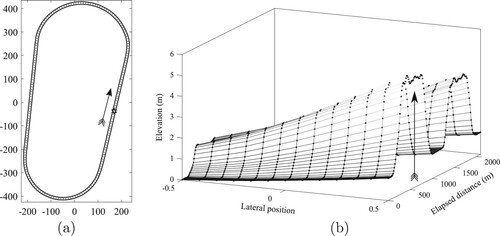
Figure 2. (a) Three-dimensional road patch and the car's position on it. (b) Road cross-section represented by $m(s,n)$, with LiDAR data points.

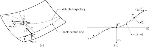
Figure 3. Heading angle χ and heading co-angle ξ.

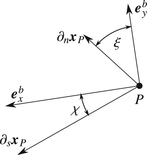
Figure 4. Centre-line curvatures for the Darlington Raceway.

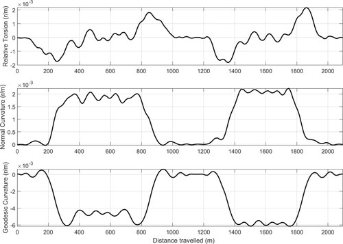
Figure 5. Darlington speedway camber variations with lateral and longitudinal positions. The track boundaries as shown solid with the centre line dot-dashed. The dotted lines are equi-spaced laterally and correspond to the survey data.

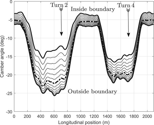
Figure 6. The (a) part of the figure shows the car's speed for the four cases described above. The (b) figure shows the engine power in the case of the optimal control simulations (left-hand axis), and the throttle opening (as a %) (right-hand axis) in the case of the measured behaviour and the industrial simulation.

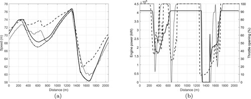
Table 1. Lap times.

Measured	30.60 s
Industrial	29.78 s
Optimal – laterally flat	30.48 s
Optimal – laterally curved	30.63 s

Figure 7. Optimal racing line. The (a) part of the figure shows the car's position in Turn 1 and the (b) part of the figure shows the car's lateral position relative to the centre line.

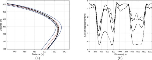
Figure 8. Normal, lateral and longitudinal tyre loads, and measured brake pressure. The industry-based simulation is shown dotted, while the optimal simulation with a laterally curved track is shown solid. The front-right tyre is blue, the front-left tyre is magenta, the rear-right tyre is black, while the rear-left tyre is shown red. (Colour online.)

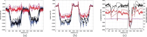
Figure 9. Front and rear ride heights. (a) The rear ride height is given by the average of the heights of chassis points $P_3$ and $P_4$ (see Figure A2). (b) The front ride height is the height of $P_5$.

Figure 10. Side-slip and roll angles on the optimal racing line. (a) The simulated (solid) and industrial (dotted) slide-slip angles. (b) The simulated (solid) and industrial (dotted) roll angles.

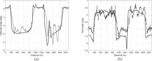
Figure 11. Optimal aerodynamic forces. (a) Drag, (b) downforce, and (c) side force; all in (N).

Figure A1. Effect of changing the car's running direction.

Table A1. Curvature and Euler angle sign changes for the opposing running direction.

$\delta (s)\to -\delta (s)$	$\tau (s)\to \tau (s)$	$\phi (s)\to -\phi (s{)}^{\mathrm{a}}$
$\dot{\delta }(s)\to -\dot{\delta }(s)$	$\dot{\tau }(s)\to \dot{\tau }(s)$	$\dot{\phi }(s)\to -\dot{\phi }$(s)
${\mathrm{\Omega }}_x(s)\to -{\mathrm{\Omega }}_x(s)$	${\mathrm{\Omega }}_y(s)\to {\mathrm{\Omega }}_y(s)$	${\mathrm{\Omega }}_z(s)\to -{\mathrm{\Omega }}_z$(s)
${\dot{\mathrm{\Omega }}}_x(s)\to -{\dot{\mathrm{\Omega }}}_x(s)$	${\dot{\mathrm{\Omega }}}_y(s)\to {\dot{\mathrm{\Omega }}}_y(s)$	${\dot{\mathrm{\Omega }}}_z(s)\to -{\dot{\mathrm{\Omega }}}_z(s)$
$a_2(s)\to a_2(s)$	$a_3(s)\to -a_3(s)$	$R_w(s)\to -R_w(s)$
${\dot{a}}_2(s)\to {\dot{a}}_2(s)$	${\dot{a}}_3(s)\to -{\dot{a}}_3(s)$	${\dot{R}}_w(s)\to -{\dot{R}}_w(s)$

${}^{\mathrm{a}}$Corrections of $\pm \pi$ radians may be required for some tracks.

Table A2. Vehicle parameters.

Symbol	Description	Value
g	Gravitational constant	9.81 m/s${}^2$
M	Vehicle mass including driver	1552.20 kg
$M_{fr}$	Target corner masses for	445.14 kg
$M_{fl}$	Suspension set up	329.28 kg
$M_{rr}$	”	282.88 kg
$M_{rl}$	”	417.79 kg
$I_{xx}$	Vehicle moments of inertia	442.85 kg m${}^2$
$I_{yy}$	”	2423.28 kg m${}^2$
$I_{zz}$	”	2616.23 kg m${}^2$
w	Vehicle length; See Figure A2	2.7895 m
a	See Figure A2	1.325 m
b	See Figure A2	1.465 m
h	Height of CoG	0.396 m
$w_f$	Front half-track width	0.778 m
$w_r$	Rear half-track width	0.783 m
$R_{fr}$	Wheel radius	0.364 m
$R_{fl}$	”	0.358 m
$R_{rr}$	”	0.361 m
$R_{rl}$	”	0.359 m
$P_{max}$	Maximum engine power	410.135 kW
ρ	Air density	1.156 kg/m${}^3$
$A_f$	Aerodynamic cross-sectional area	2.24 m${}^2$
$M_{\mathrm{arm}}$	Aerodynamic moment arm	2.794 m
$P_1$	Aero point; See Figure A2	[0.834898; 0.697738; 0.10033] m
$P_2$	”	[0.83439; $-0.6971792$; 0.08382] m
$P_3$	”	[$-0.8127492$; 0.6975856; 0.16637] m
$P_4$	”	[$-0.8134096$; $-0.6989064$; 0.1477772] m
$P_5$	”	[2.491486; 0.0004572; 0.0271272] m
$P_6$	”	[2.3992332; $-0.5836666$; 0.0195072] m
$P_7$	”	[2.3995634; 0.5846318; 0.0358648] m
$B_{\text{bal}}$	Brake balance	0.45
$K_{\text{diff}}$	Differential stiffness	2.5e4 Nms (locked differential)

Table A3. Tyre parameters.

Symbol	Front right	Front left	Rear right	Rear left
$F_{z1}$	$-$5524.54	$-$4472.44	$-$5254.62	$-$5019.47
$F_{z2}$	$-$13728.37	$-$6367.52	$-$13521.04	$-$6297.70
${\mu }_{x1}$	0.855517	1.14857	0.936367	1.160195
${\mu }_{x2}$	0.898665	1.18797	0.937544	1.186992
${\kappa }_1$	0.046921	0.04789	0.051107	0.046764
${\kappa }_2$	0.038575	0.04423	0.040467	0.044357
${\mu }_{y1}$	0.863775	1.29157	0.885916	1.198614
${\mu }_{y2}$	0.700057	1.29157	0.696319	1.065799
${\alpha }_1$	0.067888	0.05656	0.075406	0.055311
${\alpha }_2$	0.057476	0.04679	0.063077	0.050978
$Q_x$	1.498353	1.13194	1.496790	1.131497
$Q_y$	1.569762	1.34450	1.605538	1.362036

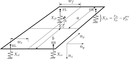
Figure A2. Chassis fixed points.

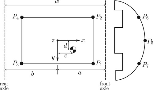
Figure A3. Aerodynamic coefficients for an optimal lap of the Darlington Raceway. The force coefficients are in black, while the moment coefficients are in blue. The x-axis is quantities are solid, the y-axis quantities are dot-dashed, and the z-axis quantities are dotted. (Colour online.)

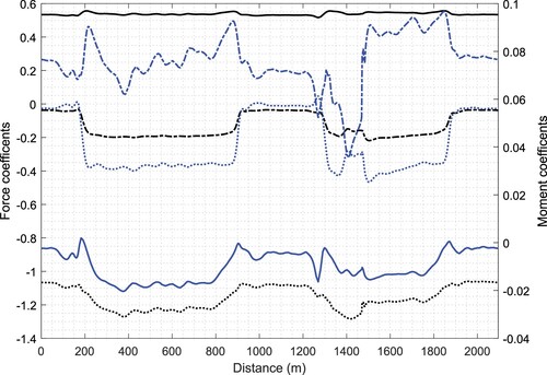
Figure A4. Rigid-chassis car with simple linear-spring suspension.