Wheel wear reduction of a mechatronic two-axle vehicle controlled with feedforward wheelset steering approaches

Figures & data

Table 1. Load collective for Metro Madrid line 10.

	NLA [m/s^2]	Curve Radius $\tilde{R}$ [m]	Cant $\tilde{h}$ [mm]	Speed $v$ [km/h]	Transition curve length ${\tilde{L}}_{tr}$ [m]	Circular curve length ${\tilde{L}}_{cr}$ [m]	Simulated distance $L^{sim}$ [m]	Cumulative length $L_{tr}+L_{cr}$ [m]	Representative share $r$ [%]
S-Curve	§	§	§	30	§	§	192	132	0.3%
	0.61	272	87	64	40	114	254	2314	5.9%
200 ≤ R ≤ 300	0.28	267	96	56	66	107	299	2273	5.8%
	−0.07	258	110	47	66	136	328	1201	3.1%
	0.70	350	53	69	55	287	457	2376	6.1%
300 < R ≤ 400	0.41	359	108	72	60	181	361	2868	7.3%
	0.13	348	131	67	67	193	387	1801	4.6%
	0.49	455	75	76	66	198	390	1152	2.9%
400 < R ≤ 600	0.21	489	93	72	87	105	339	1953	5.0%
	−0.19	502	76	45	34	76	204	788	2.0%
600 < R ≤ 800	0.46	744	25	78	63	92	278	873	2.2%
	0.06	722	42	56	42	71	215	1320	3.4%
800 < R ≤ 1200	0.31	977	10	69	33	108	234	785	2.0%
	−0.05	1067	40	54	13	47	133	220	0.6%
1200 < R ≤ 2000	0.12	1753	10	65	67	135	329	804	2.0%
Tangent	§	§	§	60	§	§	1000	9209	23.4%
	§	§	§	70 → 1	§	§	Variable	9209	23.4%

Figure 1. Nominal line 10 data: (Top) vehicle speed, (Centre) track curvature, and (Bottom) track cant. The solid line shows the nominal data while the dashed lines represent stations.

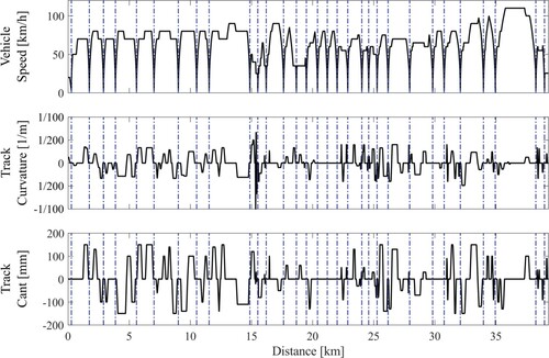
Figure 2. Line 10 statistical analysis. (A) line 10 nominal track curvature, (B) detail of the s-curve curvature, (C) occurrence of curves for curve radii greater than 200 m, and (D) K-means clustering for each curve family of (C). In (D), for each curve family, each curve is shown with a marker corresponding to the cluster it belongs to. Each cluster centroid is shown with a dashed line.

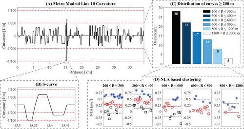
Figure 3. Wheel-rail contact conditions: (Top-left) contact overview showing the nominal wheel and rail profiles and the possible contact points, (Bottom-left) wayside lubrication showing the variation of the friction coefficient in red against the nominal rail profile in black, and (Right) equivalent conicity profile for the nominal wheel and rail condition calculated in SIMPACK. In this last, the dash-dotted line shows the conicity at 3 mm amplitude.

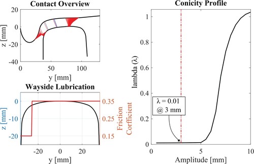
Figure 4. Track irregularities: (Left) ERRI power spectral density showing the frequency region used in the simulations, (Right) randomly generated track irregularities profiles

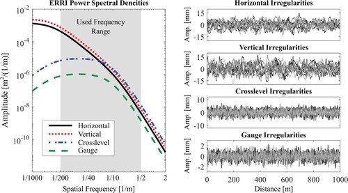
Figure 5. Mechatronic vehicle configuration: (Top) mechatronic vehicle overview, (Bottom-left) anti-roll bar motion of the U-shaped frame showing the frame deformation, and (Bottom-right) arrangement of the actuators connecting the single axle running gear to the carbody.

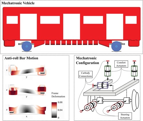
Figure 6. Control loop showing the key aspects from the multi body simulation of the vehicle in SIMPACK, through the control logic in Simulink, and to the actuator model in Simscape. Note that in the Figure (on the right) the vehicle stimuli (axlebox and carbody velocity) are provided to the left actuator while the suspension force is produced by the right actuator. This only make the figure easier to read, in the simulations all actuators receive the vehicle stimuli and produce the suspension forces.

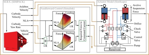
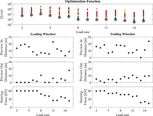
Figure 7. Optimisation overview: (Left) optimisation parameters showing the command steering force profile against the track profile, and (Right) the optimisation function showing a schematic of the leading and trailing wheelsets wear number.

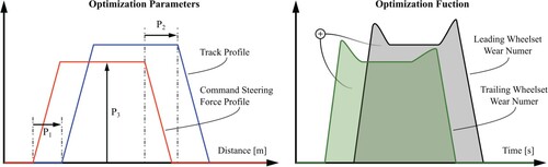
Figure 8. Difference between original feedforward controller and optimised steering controller in terms of wear number: (Left) leading wheelset, and (Right) trailing wheelset. (Top) S-curve, (Centre) Load case 2 (Table 1), and (Bottom) Load case 14 (Table 1).

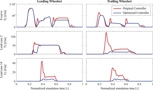
Figure 9. Dissipated energy for the first 15 load cases (the s-curve and the 14 curve load cases) comparing the standard vehicle with the mechatronic one controlled with the original controller and the optimised one. For each load case, the improvement achieved by the mechatronic vehicle with respect to the standard one is given in percentage. The average (Avg.) improvement for both controller is shown too.

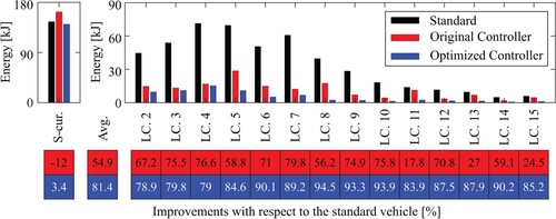
Figure 10. Comparison of measured and simulated worn wheels at the reprofiling distance of 150,000 km: (Left) leading wheelset, (Right) trailing wheelset. (Top) Wheel profiles, (Centre) wear depth, and (Bottom) error between simulated and measured wear depth.

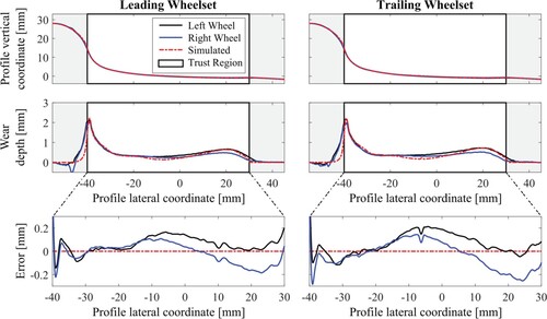
Figure 11. Wear depth comparison between the standard bogie vehicle and the mechatronic vehicle controlled with the original feedforward controller and the optimised one at the reprofiling distance of 150,000 km. (Left-top) Leading wheelset, (Left-bottom) trailing wheelset. (Right) Lost volume per vehicle and improvements in percentage of the mechatronic vehicles in comparison to the standard one.

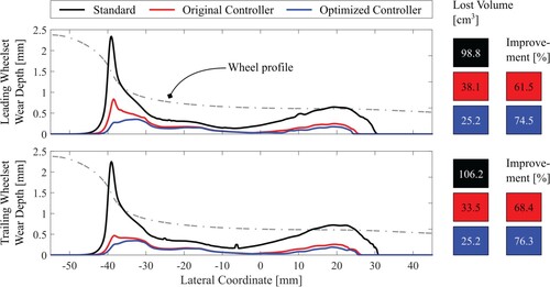
Figure 12. Sum of normal wear lost volume per load case comparing the standard bogie vehicle and the mechatronic one. (Top) Sum of lost volume, (Bottom) improvements with respect to the standard bogie in percentage.

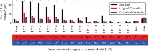
Figure 13. Comparison of improvements of the mechatronic vehicle with respect to the standard bogie vehicle calculated with $T\gamma$ based approach (energy calculation) and the ones based on the lost volume. (Top) Original feedforward controller, and (Bottom) optimised controller.

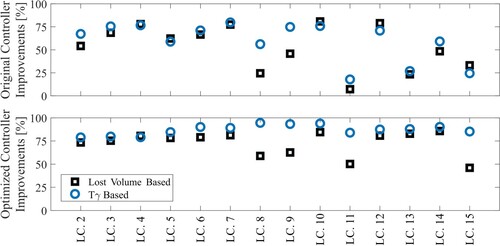
Figure A1. Results on preliminary investigation of command steering force profile timing. (Top) Steering force command, (Bottom) energy dissipation $T\gamma$. (Left) Leading wheelset, (Right) trailing wheelset.

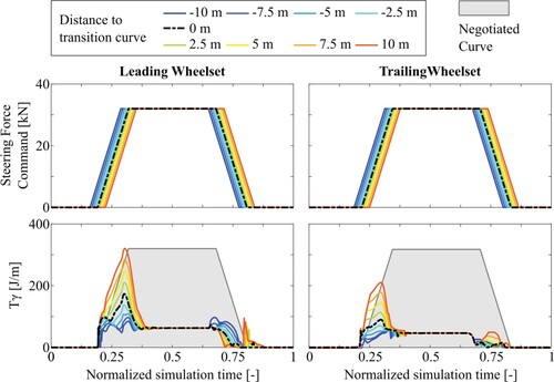
Figure A2. FAs optimisation results for the 14 curve load cases. (Top) $O_F$ for each load case showing the span of the obtained values during the optimisation procedure and the result corresponding to the final optimised value (black circle). (Left) Optimised parameters for the leading wheelset and (Right) the ones for the trailing wheelset.