Safe operating envelope based on a single-track model for yaw instability avoidance of articulated heavy vehicles

Figures & data

Figure 1. Illustrations of different yaw instabilities for a tractor (blue) and semitrailer (grey). (a) Jackknifing. (b) Trailer swing and (c) Combination spin-out.

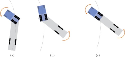
Figure 2. Free-body diagrams of the nonlinear single-track model for the AHV [23,p.296]. Forces and moments are shown in blue, velocities in green.

Figure 3. Paths followed by an AHV for two different braking manoeuvres with $V_{1x}^{\mathrm{init}}=45$ km/h, $\mu =0.3$, R = 72 m. Braking starts at $t=5\mathrm{s}$. (a) $c_{\mathrm{tractor}}=-0.8$ and $c_{\mathrm{trailer}}=0$. Jackknifing occurs and simulation is terminated when the articulation angle reaches ${90}^{\circ }$ and (b) $c_{\mathrm{tractor}}=-0.75$ and $c_{\mathrm{trailer}}=-0.75$. No yaw instability occurs and simulation is terminated when the tractor reaches zero velocity.

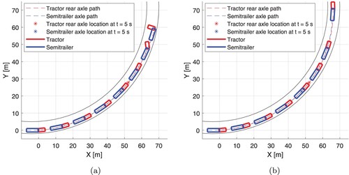
Figure 4. Eigenvalues of the linearised single-track model, actuated with five different longitudinal force pairs. $c_{\mathrm{tractor}}$ is the friction utilisation of the tractor's rear axle and $c_{\mathrm{trailer}}$ is the friction utilisation of the semitrailer's axle.

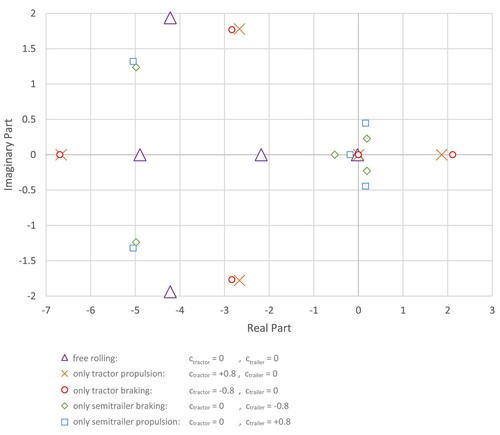
Table 1. Eigenvalues of the nonlinear single-track model actuated with 13 different longitudinal force pairs.

$c_{\mathrm{tractor}}$	$c_{\mathrm{trailer}}$	$\mathrm{Re}({\lambda }_1)$	$\mathrm{Im}({\lambda }_1)$	$\mathrm{Re}({\lambda }_2)$	$\mathrm{Im}({\lambda }_2)$	$\mathrm{Re}({\lambda }_3)$	$\mathrm{Im}({\lambda }_3)$	$\mathrm{Re}({\lambda }_4)$	$\mathrm{Im}({\lambda }_4)$	$\mathrm{Re}({\lambda }_5)$	$\mathrm{Im}({\lambda }_5)$
0	0	−4.8955	0.0000	−4.2180	1.9384	−4.2180	−1.9384	−2.1798	0.0000	−0.0235	0.0000
0.8	0	−6.6638	0.0000	−2.6662	1.7787	−2.6662	−1.7787	0.0052	0.0000	1.8667	0.0000
−0.8	0	−6.6906	0.0000	−2.8346	1.7675	−2.8346	−1.7675	0.0004	0.0000	2.1132	0.0000
0	−0.8	−4.9826	1.2370	−4.9826	−1.2370	−0.5320	0.0000	0.1893	0.2283	0.1893	−0.2283
0	0.8	−5.0477	1.3203	−5.0477	−1.3203	−0.1866	0.0000	0.1611	0.4461	0.1611	−0.4461
0.8	0.8	−6.6556	0.0000	0.0265	0.3622	0.0265	−0.3622	0.0281	0.0000	1.9497	0.0000
−0.8	−0.8	−6.6907	0.0000	−0.4781	0.0000	0.0278	0.0000	0.3745	0.0000	2.0113	0.0000
0.4	0	−4.8817	0.0000	−4.1568	1.9687	−4.1568	−1.9687	−2.2695	0.0000	−0.0236	0.0000
−0.4	0	−4.9093	0.0000	−4.2783	1.9103	−4.2783	−1.9103	−2.0921	0.0000	−0.0234	0.0000
0	−0.4	−4.9152	0.0000	−4.1930	1.9397	−4.1930	−1.9397	−2.2723	0.0000	−0.0234	0.0000
0	0.4	−4.8759	0.0000	−4.2415	1.9374	−4.2415	−1.9374	−2.0906	0.0000	−0.0237	0.0000
0.4	0.4	−4.8622	0.0000	−4.1819	1.9662	−4.1819	−1.9662	−2.1774	0.0000	−0.0238	0.0000
−0.4	−0.4	−4.9292	0.0000	−4.2549	1.9102	−4.2549	−1.9102	−2.1815	0.0000	−0.0232	0.0000

Note: Eigenvalues with the largest real part are shown in bold. Stable pairs of $c_{\mathrm{tractor}}$ and $c_{\mathrm{trailer}}$ are shown in green and unstable pairs in red colour.

Figure 5. AHV exhibiting a trailer swing due to semitrailer braking, with $c_{\mathrm{trailer}}=-0.8$ at $t=5\mathrm{s}$.

Figure 6. Changes in maximum articulation angle and side-slip angle deviations due to different values on the operational parameters: turning radius (first-row plots), initial speed (second-row plots), and friction coefficient (third-row plots) for three different braking manoeuvres. (a) $[\begin{array}{c}{c}_{\mathrm{tractor}}\\ c_{\mathrm{trailer}}\end{array}=\begin{array}{c}-0.8\\ 0\end{array}]$ (b) $[\begin{array}{c}{c}_{\mathrm{tractor}}\\ c_{\mathrm{trailer}}\end{array}=\begin{array}{c}0\\ -0.8\end{array}]$ (c) $[\begin{array}{c}{c}_{\mathrm{tractor}}\\ c_{\mathrm{trailer}}\end{array}=\begin{array}{c}-0.8\\ -0.8\end{array}]$

Figure 7. Effects of various friction utilisation ratios, $c_{\mathrm{tractor}}$ and $c_{\mathrm{trailer}}$. (a) $c_{\mathrm{tractor}}\in [-1,1]$ and $c_{\mathrm{trailer}}=0$ and (b) $c_{\mathrm{tractor}}=0$ and $c_{\mathrm{trailer}}\in [-1,1]$.

Figure 8. Maximum side-slip angle and articulation angle deviations for braking at six different speeds, according to the nonlinear single-track model.

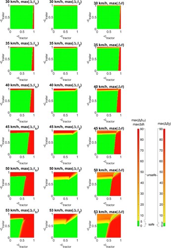
Figure 9. SOE obtained from the nonlinear single-track model of a braking AHV.

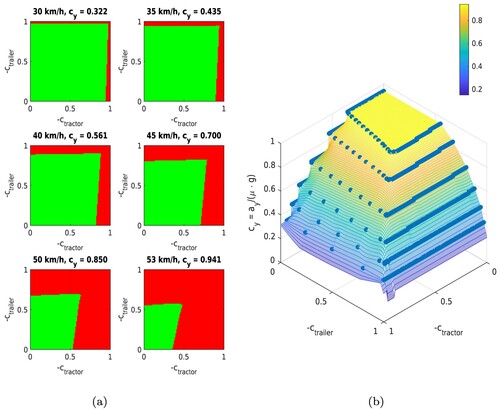
Figure 10. Different yaw instability modes shown on the SOE.

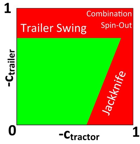
Figure 11. SOE obtained from the nonlinear single-track model of an accelerating AHV.

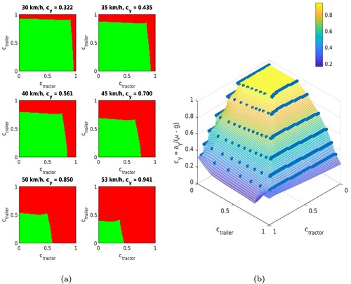
Figure 12. Slice of the SOE obtained from the nonlinear single-track model for 40 km/h ($c_y=0.561$) for any combination of propulsion and braking forces.

Table

Parameter	Description	Value	Unit
$m_1$	Mass of the tractor	12,500	kg
$m_2$	Mass of the semitrailer	13,500	kg
$J_1$	Yaw moment of inertia of the tractor	48,758	$\mathrm{kg}\cdot {\mathrm{m}}^2$
$J_2$	Yaw moment of inertia of the semitrailer	83,913	$\mathrm{kg}\cdot {\mathrm{m}}^2$
$C_{1r}$	Cornering stiffness of the rear axle of the tractor	6	–
$C_{1f}$	Cornering stiffness of the front axle of the tractor	6	–
$C_2$	Cornering stiffness of the semitrailer axle	6	–
$L_1$	Tractor wheelbase	4.085	m
$l_{1c}$	Distance between coupling to the front axle of tractor	3.7725	m
$l_{2c}$	Distance between the coupling to the semitrailer axle	7.05	m
$l_{1\mathrm{CoG}}$	Distance between the CoG and the front axle of tractor	1.534	m
$l_{2\mathrm{CoG}}$	Distance between the CoG and the semitrailer axle	1.9315	m
g	Gravitational acceleration	9.81	m/s${}^2$

Table

Parameter	Description
CoG	Centre of gravity
R	Turning radius
θ	Articulation angle
${\omega }_{\mathrm{iz}}$	Yaw rate of unit i
${\delta }_f$	Road wheel angle of the front axle
$a_{\mathrm{ij}}$	Acceleration of unit i in j direction
$P_{\mathrm{ij}}$	Coupling force at unit i in j direction
$v_{\mathrm{icj}}$	Velocity of the coupling point at unit i in j direction
$v_{\mathrm{ij}}$	Velocity of the CoG of unit i in j direction
$v_{1\mathrm{ry}}$	Lateral velocity at the rear axle of the tractor
$v_{2\mathrm{ay}}$	Lateral velocity at the semitrailer axle
$v_{1\mathrm{fjw}}$	Velocity at the front axle in j direction in the wheel coordinate frame
$v_{1\mathrm{fjv}}$	Velocity at the front axle in j direction in the vehicle coordinate frame
$s_{1\mathrm{fy}}$	Lateral slip for the front axle of the tractor
$s_{1\mathrm{ry}}$	Lateral slip for the rear axle of the tractor
$s_{2y}$	Lateral slip for the semitrailer axle
$F_{1\mathrm{fjw}}$	Front axle tyre force in j direction for the tractor
$F_{1\mathrm{rj}}$	Rear axle tyre force in j direction for the tractor
$F_{2j}$	Semitrailer axle tyre force in j direction
$F_{1\mathrm{fyw}}^{lim}$	Maximum front axle lateral tyre force for the tractor, due to friction circle
$F_{1\mathrm{ry}}^{lim}$	Maximum rear axle lateral tyre force for the tractor, due to friction circle
$F_{2y}^{lim}$	Semitrailer axle maximum lateral tyre force, due to friction circle
${\beta }_{1r}$	Side-slip angle at the rear axle of the tractor
${\beta }_2$	Side-slip angle at the semitrailer axle
μ	Friction coefficient
$c_y$	Normalised lateral acceleration

Jacobson BJH. Vehicle dynamics compendium. Gothenburg (Sweden): Chalmers University of Technology; 2020.

 Google Scholar