
Figures & data
Figure 1. Relationship between intrinsic and polar co-ordinate descriptions of a logarithmic spiral. A generic vehicle path is given by with a generic point P on it. The origin of the polar coordinate system is O, with r and φ the polar co-ordinates of P. The instantaneous centre of rotation of
at P is C. The instantaneous radius of curvature is
, with α the angle between
and the horizontal x-axis. The angles ξ and ν define the orientation of a tangent to
at P with respect to r and the x-axis respectively.
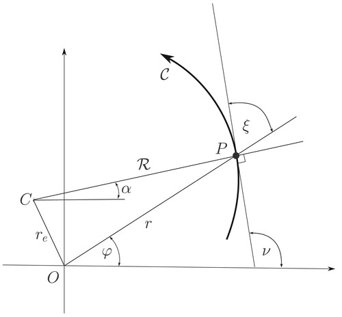
Figure 2. An exemplar test course comprising a constant radius of turn at fixed speed section OA; an accelerating straight section AB; a section BC that describes braking into a tightening turn, and a section CD requiring acceleration out of a turn that ‘opens up’.
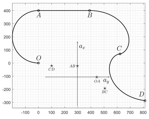
Table 1. Drivability metric.
Figure 3. Abstract GG diagram with its periphery described in terms of polar coordinates.
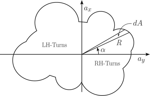
Figure 4. Kinematics of a single-track car model showing its basic geometric parameters [Citation3].
![Figure 4. Kinematics of a single-track car model showing its basic geometric parameters [Citation3].](/cms/asset/14b7519d-dfb4-4c88-9ab5-1fe335171f36/nvsd_a_2379532_f0004_ob.jpg)
Figure 5. Single-track car model operating at different speeds on inclined planar road surfaces. The left-hand figure shows the vehicle GGV diagram on a horizontal road surface at 70 m/s (red), 50 m/s (black) and 30 m/s (blue). The central figure shows the vehicle operating at 50 m/s on an inclined road surface with a inclination angle (red), a level road surface (black), and a
declination angle (blue). The right-hand figure shows that vehicle operating at 50 m/s on a cambered road surface with a
camber angle (blue), a level road surface (black), and a
camber angle (red).
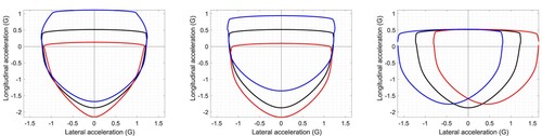
Figure 6. Single-track car model operating at 50 m/s on a horizontal road surface. The left-figure shows the front (red) and rear (blue) tyre cornering stiffnesses and the vehicle understeer coefficient (black). The right-hand figure shows the two-state linear model eigenvalues evaluated on the periphery of the GG diagram; the real parts are shown red and the imaginary parts blue.
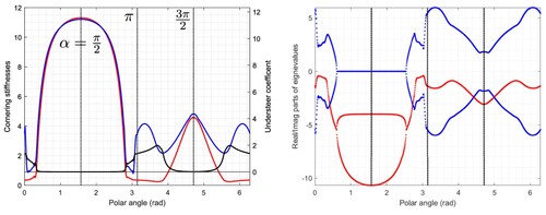
Figure 7. Stability eigenvalues on the periphery of the GG diagram at 50 m/s on a planar road surface. The real parts of the linearised model eigenvalues are shown in red, while the imaginary parts are illustrated in blue. The left-hand diagram corresponds to a road cambered at , the central plot is for a level road surface, while the right-hand diagram is for a road cambered at
.
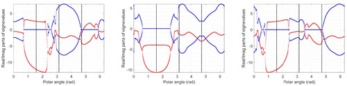
Figure 8. Steady-state gain of the transfer function from the steering angle to the yaw rate for the vehicle operating at 50 m/s on a horizontal road surface.
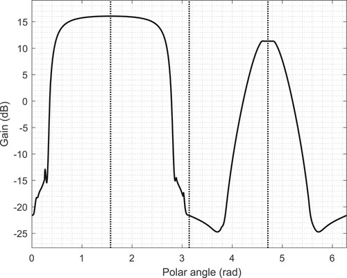
Figure 9. GGV diagrams for a Gen-7 NASCAR operating on planar road surfaces of variable lateral road camber; the left-hand figure is for of camber, the centre figure is for a horizontal road surface and the right-hand figure is for
of lateral road camber. The black plots correspond to the car travelling at 80 m/s; the red curves correspond to 70 m/s; the blue curves correspond to 60 m/s; the magenta curves are for 50 m/s and the green curves are for 40 m/s.
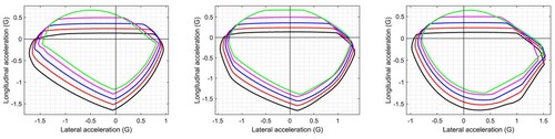
Figure 10. Normal and lateral tyre loads as a function of the GG diagram sweep angle . The lateral acceleration is
and the camber angle ϕ. All the car parameters are assumed normalised so that g = 1, M = 1, and R is in G's. All lengths are given as fractions of the vehicle length.
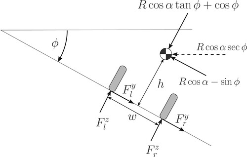
Table 2. Idealised and normalised tyre loading parameters.
Figure 11. Total lateral tyre loads as a function of the sweep and camber angles, respectively α and ϕ. All the car parameters are assumed normalised so that g = 1, M = 1, and R is in G's. The black curve corresponds to . The red curve is for
, while the blue curve represents the
case.
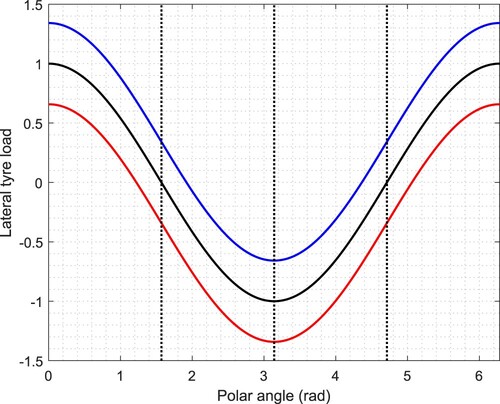
Figure 12. Idealised left- and right-hand tyre normal loads for varying road camber; the left-hand plot is for the left-hand tyre. The black curves are for a level road. The red curve represents a road camber of , while the blue curve is for a road camber of
.
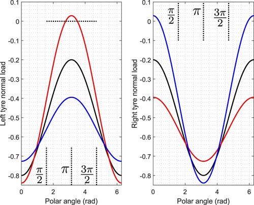
Figure 13. Tyre normal loads for a Gen-7 NASCAR travelling at 50 m/s. The black plot corresponds to the car operating on a horizontal road surface. The red plot corresponds to the car operating on a road surface with of camber. The blue plot corresponds to the car operating on a road surface with
of camber.
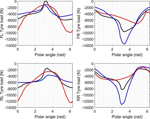
Figure 14. GGV diagrams for a Gen-7 NASCAR operating on a conical road surface with a camber angle of . The black plots corresponds to the car travelling at 80 m/s; the red curves corresponds to 70 m/s; the blue curves corresponds to 60 m/s; the magenta curves are for 50 m/s and the green curves are for 40 m/s.
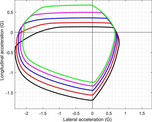
Figure 15. Measured normal tyre loads captured on an instrumented Gen-6 NASCAR on the Darlington Raceway.
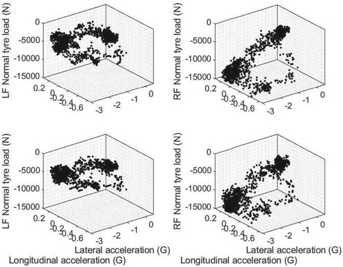
Figure 16. Measured lateral and longitudinal accelerations captured on an instrumented Gen-6 NASCAR on the Darlington Raceway.
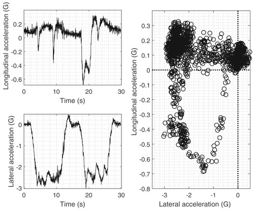
Figure 17. Eigenvalue plots for a Gen-7 NASCAR operating at 50 m/s on a conical road surface. The real parts of the linearised model eigenvalues are shown in red, while the imaginary parts are illustrated in blue. The black dot-dash curve is the maximum achievable acceleration as the GG diagram is traversed. The left-hand figure is for of road camber, the central figure is for a horizontal road surface and the right-hand figure is for
of camber.
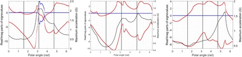
Figure 18. Steady-state steer angle gains for a Gen-7 NASCAR operating at 50 m/s on a horizontal planar road surface. The left-hand figure is the yaw-rate gain, while the right-hand figure is the side-slip angle gain.
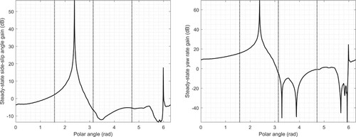
Figure 19. Brake balance for a Gen-7 NASCAR travelling at 50 m/s. The left-hand figure is for a level road surface. The right-hand figure is for a curved road surface with of camber. The black plot corresponds to the car operating with 67% of the braking torque applied to the front axle. The red plot corresponds to the car operating with 80% of the braking torque applied to the front axle. The blue plot corresponds to the car operating with 90% of the braking torque applied to the front axle.
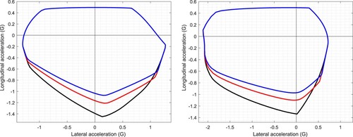
Figure 20. Stability due to variable brake balance for a Gen-7 NASCAR travelling at 50 m/s on a level road surface. The real parts of the linearised model eigenvalues are shown in red, while the imaginary parts are illustrated in blue. The black dot-dash curve is the maximum achievable acceleration as the GG diagram is traversed. The left-hand figure corresponds to a nominal brake balance of 67% on the front wheels. The central figure corresponds to a nominal brake balance of 80% on the front wheels. The right-hand figure corresponds to a nominal brake balance of 90% on the front wheels.
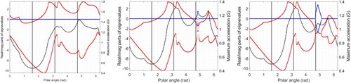
Table B1. Single-track car model parameters.
Table B2. Single-track car model parameters.