Figures & data
Figure 1. Location map. The outlined area in pale blue is the best estimate of the River Çarşamba catchment area producing flow to the area of the site in the Neolithic (see Wainwright and Ayala Citation2021] for details).
![Figure 1. Location map. The outlined area in pale blue is the best estimate of the River Çarşamba catchment area producing flow to the area of the site in the Neolithic (see Wainwright and Ayala Citation2021] for details).](/cms/asset/a60845b8-f00c-446c-9b73-a77ecdd47250/rwar_a_2125058_f0001_oc.jpg)
Figure 2. Image of a dryland anastomosing channel (from North, Nanson, and Fagan Citation2007) and a typical cross section, showing multiple channel threads, “islands” and riparian vegetation. The photograph is of Copper Creek, Queensland, Australia, with a similar mean annual rainfall to the Konya Plain, albeit with higher mean annual temperatures.
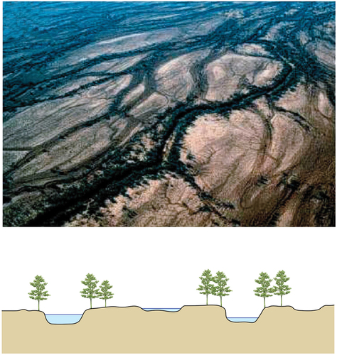
Figure 3. Crop-Growth cycle for winter-sown wheat compared to the climatogram for modern Çatalhöyük (based on the CRU-TS 4 reconstruction of Harris et al. Citation2020) and to modern baseline flows for the River Çarşamba without recent historical catchment modifications (based on Wainwright and Ayala Citation2021). Blue arrows show periods of time when soil moisture is critical for crop growth and production. The shaded areas on the climatogram show 95% confidence intervals for precipitation and temperature based on the time-series record from 1901 to 2016. The flow summary plot shows the 95% confidence interval as well as monthly mean and maximum values, derived from multiple flow simulations to allow propagation of uncertainty from the climate data through the HEC-HMS rainfall-runoff model used to estimate flows (see Wainwright and Ayala Citation2021 for further details).
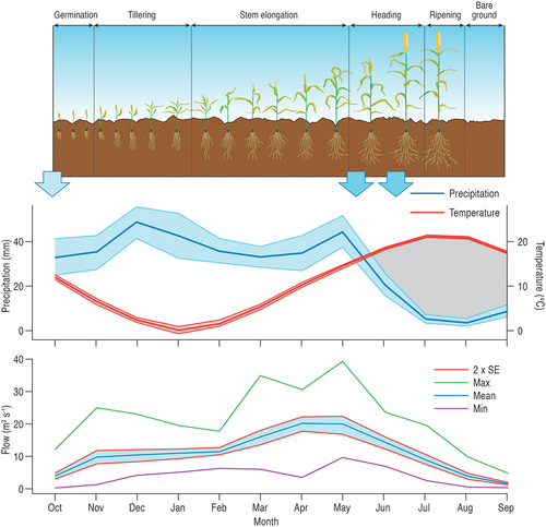
Table 1. Seasonality data for winter-sown crops in the Greater Konya Basin.
Figure 4. Climatogram for Climate Scenario 2 with moderate woodland in the catchment and the resulting simulated flow regime. The climate scenario accounts for uncertainties in the original proxy and the process of extrapolation to the catchment area, and 95% confidence limits are estimated using Monte Carlo simulations using a stochastic daily weather generator; Monte Carlo simulations are then used to propagate these values through the HEC-HMS rainfall-runoff model, with the shaded blue area showing the 95% confidence interval, and simulated monthly minimum and maximum values also plotted (see Wainwright and Ayala Citation2021 for details).
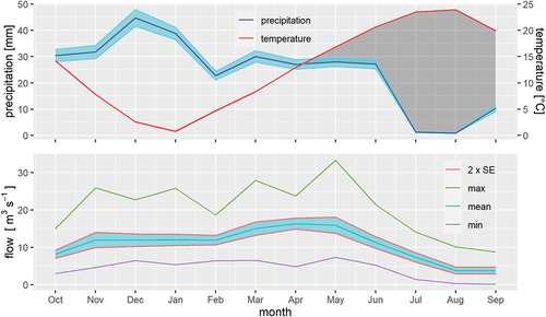
Figure 5. Climatogram for Climate Scenario 14 with moderate woodland in the catchment and the resulting simulated flow regime. The uncertainties are represented as outlined in the caption to (see Wainwright and Ayala Citation2021 for details).
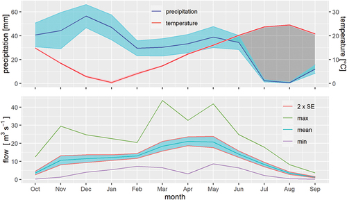
Figure 6. Simulation of the water-table depth across the floodplain for the modern baseline scenario. The channel is on the right-hand edge (at a distance of 3 km), and the x values represent the distance from the simulation edge on the left-hand side. This section can be considered symmetrical about the channel belt because of the assumptions made in the model, so only one side is shown. Note that the distances in the graphic are irregular to pick out where major changes occur. The box-and-whisker plots are used to show the effect of propagating the climate and flow uncertainties through the model using Monte Carlo simulations. The solid brown line is the ground surface, and the dashed brown lines are at 0.2 m and 1.0 m to represent likely rooting depths at key points in the agricultural cycle.
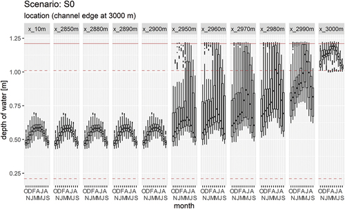
Figure 7. Simulation of the water-table depth across the floodplain for Climate Scenario 2 with moderate woodland in the catchment. Distances are the same as in , and uncertainties represented in the same way. The solid brown line is the ground surface, and the dashed brown lines are at 0.2 m and 1.0 m to represent likely rooting depths at key points in the agricultural cycle.
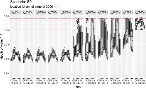
Figure 8. Simulation of the water-table depth across the floodplain for Climate Scenario 14 with moderate woodland in the catchment. Distances are the same as in , and uncertainties represented in the same way. The solid brown line is the ground surface, and the dashed brown lines are at 0.2 m and 1.0 m to represent likely rooting depths at key points in the agricultural cycle.
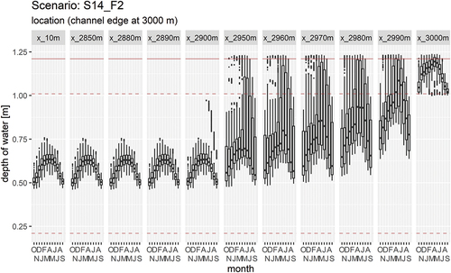
Figure 9. Areas of potential agricultural use suggested by the cost-surface analysis. Zones around the site. The 0.5-h and 2-h walking times use the Tobler off-path function with double resistance for the channel belt. The position of the main channel belt is a best estimate from stratigraphy (see Ayala et al. Citation2017, Citation2021), and the lighter shaded channel belt is the branch to Lake Hotamiş based on de Meester (Citation1970) but evidence that it was active in Neolithic is limited. The buffer zone on the channel belt is based on the Boussinesq analyses ().
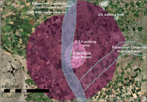
Figure 10. Schematic cross-section of the channel belt showing typical water depths at the wettest and driest points in the hydrological year.
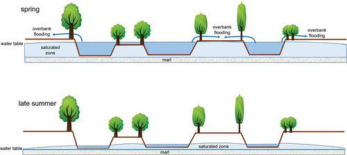
Figure 11. Simplified spatial distribution of possible agroeconomic settings around Neolithic Çatalhöyük.
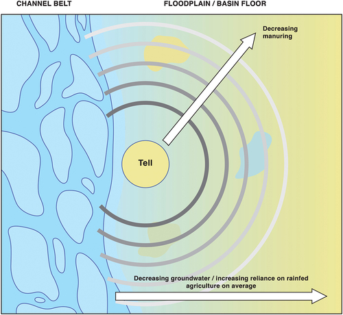
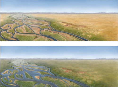
Figure 12. Bird’s-Eye view of reconstruction of the Çatalhöyük landscape, looking south-west (illustration by Katy Killackey): a. dry season (late summer), b. wet season (spring).