Animal- and herd-level factors associated with onset of puberty in grazing dairy heifers

Figures & data

Table 1. Descriptive statistics of grazing heifers (n = 5,004) from 54 dairy herds that had puberty traits collected on three occasions at approximately 10 (visit 1; V1), 11 (visit 2; V2) and 12 months of age (visit 3; V3).

	Mean	SD	Median	Range	Missing values
Animal characteristics
% Holstein	52	12.3	52.1	0–90.2	295
% Friesian	34	9.9	34.5	0–75.5	295
% Jersey	13	13.0	9.3	0.1–100	295
% Ayrshire	1	2.3	0.6	0–87.5	295
Animal measures
Age at V1 (days)	299	14.4	299	236–347	–
Age at V2 (days)	327	14.5	327	264–374	–
Age at V3 (days)	355	14.6	355	292–403	–
Height at V2 (cm)	115	4.8	115	91–132	22
Length at V2 (cm)	105	5.9	105	80–135.5	22
AGD at V2 (mm)	81	10.3	81	45–124	23
Liveweight at V2 (kg)	226	34.1	225	119–350	86
PMLWT	0.43	0.61	0.42	0.22–0.66	445
Liveweight BV	29.4	20.0	29.0	−76.7–93.4	378
% of heifers pubertal by V1	20	39.7	–	3.8–31.3^a	39
% of heifers pubertal by V2	39	48.7	–	16.6–55.6^a	51
% of heifers pubertal by V3	56	49.7	–	33.4–79.8^a	26
Age at puberty (days)^b	352	34.9	359.0	251–429	26

^a IQR for the percentage of animals pubertal by each visit.

^b Right censored; animals that did not reach puberty before V3 were assigned an age at puberty of their age at V3 + 31 days.

AGD = anogenital distance; BV = breeding value; PMLWT = proportion of mature liveweight.

Figure 1. Proportion of Holstein (black), Friesian (grey) and Jersey (white) breeds represented in dairy heifers (n = 5,004) from herds (n = 54) in North Waikato, South Waikato, Taranaki, and North Otago regions included in a study of risk factors associated with the onset of puberty.

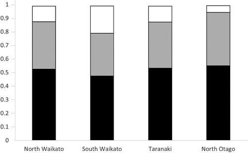
Table 2. Individual risk factors associated with the likelihood of an animal reaching puberty in a population of 5,004 grazing heifers across 54 herds. Fifteen separate multivariable logistic regression model outputs for the effects of liveweight, height, length, anogenital distance (AGD), or proportion of mature liveweight (PMLWT) measured at visit 2 (V2) are presented for the chance of an animal being pubertal or not by visit 1 (V1), visit 2 (V2) or visit 3 (V3), after adjusting for age at V2, and Holstein and Jersey breed proportions, with herd included as a random effect (for each model).

Visit^a	Predictor^b	Estimated coefficient		P-value	Relative risk^c		Unit^d
		Mean	SEM		Mean	95% CI
V1
	Liveweight (kg)	0.02	0.002	<0.001	1.200	1.162–1.239	10 kg
	PMLWT	14.28	1.199	<0.001	1.120	1.099–1.141	1%
	Height (cm)	0.03	0.012	0.007	1.026	1.007–1.045	1 cm
	Length (cm)	0.06	0.010	<0.001	1.046	1.030–1.061	1 cm
	AGD (mm)	0.00	0.005	0.507	1.028	0.948–1.113	10 mm
V2
	Liveweight (kg)	0.03	0.002	<0.001	1.169	1.145–1.193	10 kg
	PMLWT	16.62	1.092	<0.001	1.103	1.090–1.117	1%
	Height (cm)	0.05	0.010	<0.001	1.033	1.021–1.045	1 cm
	Length (cm)	0.06	0.008	<0.001	1.038	1.028–1.048	1 cm
	AGD (mm)	0.00	0.004	0.344	1.025	0.973–1.079	10 mm
V3
	Liveweight (kg)	0.03	0.002	<0.001	1.135	1.118–1.151	10 kg
	PMLWT	18.79	1.126	<0.001	1.082	1.072–1.091	1%
	Height (cm)	0.07	0.010	<0.001	1.029	1.021–1.038	1 cm
	Length (cm)	0.07	0.008	<0.001	1.032	1.025–1.040	1 cm
	AGD (mm)	0.02	0.004	<0.001	1.085	1.048–1.122	10 mm

^a Visits occurred when animals were approximately 10 (V1), 11 (V2) and 12 (V3) months of age.

^b Predictor measured at V2.

^c Relative risks were calculated (Zhang and Yu 1998), where p = risk in the pre-pubertal group:$\mathrm{Relative}\mathrm{risk}=\mathrm{OR}÷(1-\rho )+(\rho \times \mathrm{OR})$.

^d Relative risk indicates the probability of the outcome occurring in the heifers that have reached puberty compared with pre-pubertal heifers (referent group). Relative risk is adjusted according to the specified unit for each predictor variable, e.g. the relative risk of being pubertal at V1 presented for liveweight at V2 is based on a 10 kg increase in mean liveweight at V2.

Table 3. Combined risk factors associated with the likelihood of an animal reaching puberty in a population of 5,004 grazing heifers across 54 herds. Multivariable logistic regression model outputs for the effects of age at visit 2 (V2), Holstein and Jersey breed proportions, liveweight, height, length, anogenital distance (AGD), and proportion of mature liveweight (PMLWT) on the chances of an animal being pubertal at visit 1 (V1), V2 or visit 3 (V3) with herd included as a random effect.

Visit^a	Predictor	Estimated coefficient			Relative risk^b
		Mean	SEM	P-value	Mean	95% CI
V1
	Age at V2	0.02	0.005	<0.001	1.141	1.064–1.221
	Holstein breed proportion	−0.39	0.598	0.510	0.969	0.880–1.064
	Jersey breed proportion	2.43	0.540	<0.001	1.210	1.115–1.310
	Liveweight	0.03	0.003	<0.001	1.213	1.166–1.261
	Height	−0.03	0.013	0.011	0.756	0.603–0.940
	Length	0.01	0.011	0.205	1.116	0.941–1.314
	AGD	−0.01	0.005	0.687	0.983	0.905–1.067
	PMLWT^c	15.31	1.418	<0.001	1.129	1.105–1.154
V2
	Age at V2	0.03	0.004	<0.001	1.162	1.114–1.210
	Holstein breed proportion	−0.32	0.495	0.515	0.980	0.922–1.040
	Jersey breed proportion	2.53	0.466	<0.001	1.159	1.101–1.217
	Liveweight	0.03	0.002	<0.001	1.169	1.140–1.198
	Height	−0.02	0.011	0.152	0.901	0.775–1.037
	Length	0.01	0.009	0.150	1.084	0.970–1.200
	AGD	−0.01	0.004	0.667	0.988	0.935–1.042
	PMLWT^c	16.67	1.282	<0.001	1.104	1.088–1.120
V3
	Age at V2	0.03	0.004	<0.001	1.108	1.077–1.138
	Holstein	−1.04	0.493	0.034	0.954	0.910–0.997
	Jersey breed proportion	2.04	0.461	<0.001	1.089	1.050–1.127
	Liveweight	0.03	0.002	<0.001	1.129	1.109–1.148
	Height	−0.01	0.012	0.276	0.944	0.843–1.044
	Length	0.02	0.009	0.036	1.085	1.006–1.162
	AGD	0.01	0.005	0.003	1.059	1.020–1.097
	PMLWT^c	18.12	1.314	<0.001	1.079	1.068–1.090

^a Visits occurred when animals were approximately 10 (V1), 11 (V2) and 12 (V3) months of age.

^b Relative risk indicates the probability of the outcome occurring in the heifers that have reached puberty compared with pre-pubertal heifers (Referent group). Relative risks were calculated (Zhang and Yu 1998), where p = risk in the pre-pubertal group: $\mathrm{Relative}\mathrm{Risk}=\mathrm{Odds}\mathrm{Ratio}÷(1-\rho )+(\rho \times \mathrm{Odds}\mathrm{Ratio})$.

^c Results for proportion of mature liveweight (PMLWT) are based on a second, similar model that included all other risk factors except for liveweight.

Table 4. Results of Cox proportional hazards model and HR (95% CI) for the effect of liveweight, proportion of mature liveweight (PMLWT), height, length and anogenital distance (AGD) on the hazard of puberty for dairy heifers (n = 5,004, from 54 herds). Age at visit 2 (V2; approximately 11 months of age) and proportion Holstein and Jersey were included in the model as potential confounders and herd was included as the random effect.

Predictor	Estimated coefficient			Hazard ratio		Unit
	Mean	SEM	p-value	HR	95% CI
Age at V2	−0.01	0.002	0.229	0.975	0.935—1.017	10 days
Holstein breed proportion	−0.55	0.277	0.048	0.947	0.897—1.000	0.1
Jersey breed proportion	1.56	0.260	<0.001	1.169	1.111—1.230	0.1
Liveweight	0.02	0.001	<0.001	1.186	1.158—1.215	10 kg
Height	−0.01	0.006	0.139	0.912	0.806—1.031	10 cm
Length	0.01	0.005	0.130	1.078	0.978—1.189	10 cm
AGD	0.01	0.002	0.1151	1.039	0.990—1.091	10 mm
PMLWT^a	10.2	0.652	<0.001	1.108	1.094—1.122	0.01

^a Results for PMLWT are based on a second, similar model that included other risk factors except for liveweight.

Figure 2. Cumulative percentage of heifers (n = 5,004) within each of the 58 heifer groups that had elevated blood progesterone (>1 ng/mL) indicating puberty attained by visit 1 (black; heifers approximately 10 months old), visit 2 (grey; heifers approximately 11 months old) or visit 3 (white; heifers approximately 12 months old).

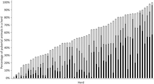
Table 5. Herd-level risk factors influencing the proportion of heifers in a dairy herd that had reached puberty when the mean age of heifers (n = 5,004, from 54 herds) was 299 days (at visit 1^a). Partial least squares model outputs are presented including raw and standardised regression coefficients, and variable importance in projection (VIP) values for the first component.

Variable	Raw coefficient	Standardised coefficient	VIP^b
Intercept	−0.864	0.000	–
Jersey breed proportion	0.274	0.108	0.397
Holstein breed proportion	−0.427	−0.171	0.643
Weighing frequency	−0.027	−0.143	0.762
Heifers reaching targets	0.104	0.168	0.764
Vaccination (leptospirosis)	0.064	0.111	0.774
SD of herd PMLWT	0.236	0.008	0.815
Supplements (preferential feeding)	−0.093	−0.182	0.876
SD of herd liveweight	0.002	0.038	0.979
Mean herd liveweight	0.002	0.287	1.541
Mean herd PMLWT	1.459	0.349	1.703

^a Heifers were approximately 10 months of age.

^b Indicates the influence of predictor variables on the model. A greater VIP indicates that a variable has a greater contribution towards the y variance explained by the model.

PMLWT = proportion of mature liveweight.

Table 6. Herd-level risk factors influencing the proportion of heifers in a dairy herd that had reached puberty when the mean age of heifers (n = 5,004, from 54 herds) was 327 days (at visit 2^a). Partial least squares model outputs are presented including raw and standardised regression coefficients, and variable importance in projection (VIP) values for the first component.

Variable	Raw coefficient	Standardised coefficient	VIP^b
Intercept	−1.376	0.000	–
Region (North Otago)	−0.048	−0.056	0.406
Supplements (offered regardless of season)	0.062	0.111	0.653
Region (South Waikato)	−0.149	−0.270	0.671
Weighing frequency	−0.008	−0.032	0.676
Region (Taranaki)	0.014	0.020	0.676
Jersey breed proportion	0.226	0.070	0.702
SD of herd PMLWT^a	4.411	0.118	0.724
Holstein breed proportion	−0.634	−0.201	0.776
Heifers reaching targets	0.039	0.050	0.826
Land type (steep)	−0.204	−0.195	0.844
Land type (rolling)	0.063	0.112	0.862
SD of herd liveweight	0.005	0.073	0.955
Supplements (preferential feeding)	−0.121	−0.187	0.980
Mean herd liveweight	0.004	0.384	1.869
Mean herd PMLWT	2.338	0.442	1.980

^a Heifers were approximately 11 months of age.

^b Indicates the influence of predictor variables on the model. A greater VIP indicates that a variable has a greater contribution towards the y variance explained by the model.

PMLWT = proportion of mature liveweight.

Table 7. Herd-level risk factors influencing the proportion of heifers in a herd that had reached puberty when the mean age of heifers (n = 5,004, from 54 herds) was 355 days (at visit 3^a). Partial least squares model outputs are presented including raw and standardised regression coefficients, and variable importance in projection (VIP) values for the first component.

Variable	Raw coefficient	Standardised coefficient	VIP^b
Intercept	−1.016	0.000	–
Jersey breed proportion	0.180	0.057	0.547
Holstein breed proportion	−0.177	−0.057	0.570
Heifers reaching targets	0.106	0.139	0.662
Vaccination (Rotavirus)	0.094	0.156	0.675
Land type (steep)	−0.140	−0.137	0.693
Weighing frequency	−0.022	−0.096	0.712
Supplements (offered regardless of season)	0.055	0.100	0.725
Land type (rolling)	−0.022	−0.040	0.818
SD of herd liveweight	0.006	0.087	0.827
Supplements (preferential feeding)	−0.128	−0.203	0.960
Mean herd liveweight	0.003	0.330	1.815
Mean herd PMLWT	1.822	0.352	1.844

^a Heifers were approximately 12 months of age.

^b Indicates the influence of predictor variables on the model. A greater VIP indicates that a variable has a greater contribution towards the y variance explained by the model.

PMLWT = proportion of mature liveweight.

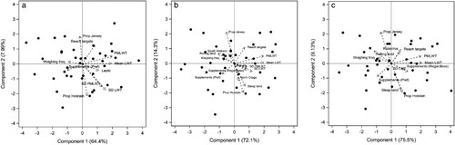
Figure 3. Correlation loading plots for the partial least squares (PLS) model of herd-level risk factors influencing the proportion of heifers in a herd that had reached puberty by (a) visit 1 (heifers approximately 10 months old), (b) visit 2 (heifers approximately 11 months old), and (c) visit 3 (heifers approximately 12 months old). Component 1 explains a proportion of the variation in the response, and the variables furthest from 0 along the x-axis (a greater X-loading value) have the greatest influence (represented by the vector arrows). Component 2 explains an additional proportion of the variation in the response and the variables furthest from 0 along the y-axis have the greatest influence (represented by the vector arrows). The vector arrows represent the X-loadings (at 4× scale for ease of interpretation) for each predictor that comprises each PLS component. The black dots represent the X-scores for each herd.

Zhang J, Yu KF. What’s the relative risk? A method of correcting the odds ratio in cohort studies of common outcomes. Journal of the American Medical Association 280, 1690–1, 1998. https://doi.org/10.1001/jama.280.19.1690

 PubMed Web of Science ®Google Scholar