
Figures & data
Figure 1. A) The geographic region surrounding the archaeological site of Dhiban, with site location marked. B) The archaeological site of Dhiban. Excavation units (5 × 5 m) are outlined in white, and adjacent labels name each excavation area. The topographic lines are at an interval of 15 m.
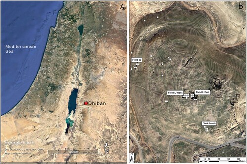
Figure 2. The collapsed room in Field S in 2013. Unit boundaries have been superimposed on their approximate locations as dashed black lines (photo credit: John E. Webley). The dashed white lines indicate hypothesized arch locations on each set of springers. The numbers indicate 1) arch springers, 2) fallen paving stones, and 3) a drain-like feature. Breakout boxes illustrate B) extensive ash and burning visible on architecture (AX55/AW54) and C) large quantities of pottery, especially storage vessels, recovered from the southern portion of Unit AW54 between A:2 and A:1.
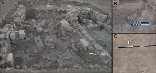
Figure 3. A) Calibrated radiocarbon probability distributions arranged according to their depth (y-axis) and by excavation unit. B) Bayesian modeled start and end date boundaries for the collapse context (see Supplemental Material 1). C) Spatial locations of calibrated dates within both phases of architecture (post-collapse: gray, collapse: unfilled lines), with rooms or areas highlighted and labeled.
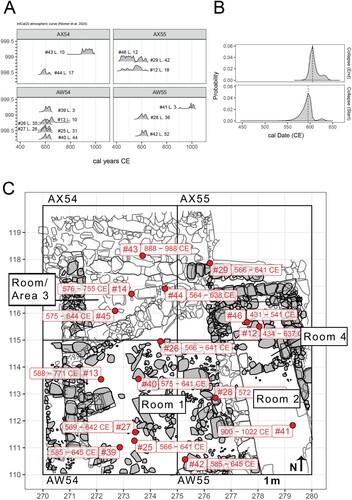
Table 1. Uncalibrated and calibrated radiocarbon dates collected from archaeological plant remains in Field S deposits up to the 2017 season. Calibrated dates are based on the IntCal20 curve and were calibrated in R using the rcarbon package. For modeled dates, see Supplemental Material 1.
Table 2. The count, proportion, and ubiquity of major classes of archaeobotanical remains recovered in Field S by Room/Area.
Figure 4. The spatial distribution of the densities of crop remains (grains, seeds, etc. per L) recovered in each flotation sample. Each point represents a bulk flotation sample, and its size is proportional to the density of remains. Color symbolizes the Gi* statistic. Representative photos of specimens of each type of crop remain are located to the right of each plot.
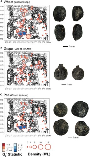
Figure 5. The vertical location of each bulk flotation sample, where the y-axis represents depth (in cm), and the x-axis represents northing and southing values (in m). The figure in the bottom-left indicates the direction of view across excavation units. Point sizes are proportional to the combined density of wheat, pea, and grape remains. Points are colored according to the relative percentage of each taxon they contain. The none category indicates none of the three remains was present. All radiocarbon dates are calibrated to 1.
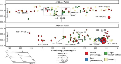
Figure 6. A) Density of ceramic remains (g/L) recovered in the heavy fraction of flotation samples. The size of points and color (including the 1 × 1 m grids) indicates the density of remains. B) Images of objects include 1) a basalt quern, 2) an entire juglet recovered in situ, 3) a ceramic cross, 4) an as-yet-unidentified carbonized larva, and 5) and 6) are a reconstructed pouring and cooking vessel, respectively (assembled at UCLA by Francisca Bravo, Cassandra Dadat, and Kaitlyn Ireland under the supervision of Vanessa Muros). The locations of these items are indicated on the map by their associated number.

Figure 7. The distribution of all grape remains recovered in flotation samples from the collapse deposits, in which point size is proportional to the total density of grape pips, pedicels, and pressed skins. The interior colors represent the relative percentage of each recovered item, and images of representative archaeological remains are located beneath the legend.
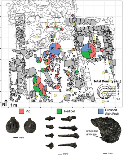
Figure 8. The ubiquity, or proportional presence across samples, of selected crop remains from sites near Dhiban that date approximately between a.d. 500 and 700 where such data are available. The number of analyzed samples is located with each plot.
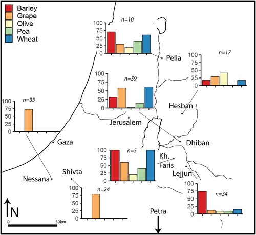
Table 3. Contemporaneous sites in the southern Levant ca. 6th/7th century a.d. that have reported relevant archaeobotanical data. A ‘+’ indicates the presence of that archaeobotanical remain category. Sites are arranged according to their direct linear distance in kilometers from Dhiban.