Figures & data
Figure 1. (a) A single example of a proposed CD from Equation (Equation2(2)
(2) ) generated from
. The confidence level required to bound the true mean
in this example is shown as 0.65. (
![]()
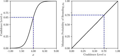
Figure 2. (a) A single example of a proposed CD from Equation (Equation6(6)
(6) ) generated from
. The confidence level required to bound the true rate
is shown as 0.75. (
![]()
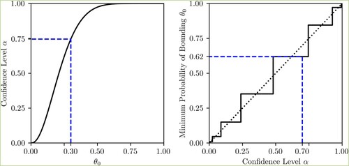
Figure 3. (a) A single example of a proposed CD from Equation (13) generated from . The confidence level required to bound the true rate
is shown as [0.05, 0.17]. (
![]()
![Figure 3. (a) A single example of a proposed CD from Equation (13) generated from x={x1,…,x10}∼Ber(p=θ0). The confidence level required to bound the true rate θ0 is shown as [0.05, 0.17]. (Display full size, CU∗(θ,x); Display full size, CL∗(θ,x); Display full size, C∗(θ0,x)). (b) Singh plot for the proposed CD about the same target distribution, generated from m=104 samples X={x1,…,xm}. (Display full size, SU(α;θ0); Display full size, SL(α;θ0); Display full size, U(0,1); Display full size, S(α=0.7;θ0)).](/cms/asset/979e9641-d74e-4191-8019-c5d1addad1ed/gscs_a_2044814_f0003_oc.jpg)
Figure 4. (a) A single example of a proposed CD from Equation (14) generated from where
. The confidence level required to bound the true value
is shown as
. (
![]()
![Figure 4. (a) A single example of a proposed CD from Equation (14) generated from x={x1,…,x10}∼F([μ1,μ2],[σ1,σ2]) where F([μ1,μ2],[σ1,σ2])=0.5⋅N(μ1=4,σ1=3)+0.5⋅N(μ2=5,σ2=1.5). The confidence level required to bound the true value xn+1 is shown as C(μ0,x)=[0.55,0.64]. (Display full size, CU∗(θ,x); Display full size, CL∗(θ,x); Display full size, C∗(θ0,x)). (b) Singh plot for the proposed imprecise CD about the same target distribution, generated from m=104 samples X={x1,…,xm} (Display full size, SU(α;θ0); Display full size, SL(α;θ0); Display full size, U(0,1); Display full size, S(α=0.7;F([μ1,μ2],[σ1,σ2]))).](/cms/asset/2d934fb6-ac0f-4fd4-87c0-48cba8991237/gscs_a_2044814_f0004_oc.jpg)
Figure 5. A series of Singh plots used for inference about generated using Equation (13) from
samples of varying length n (
![]()
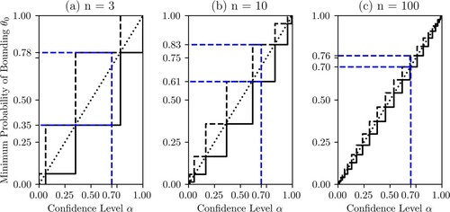
Figure 6. A series of Singh plots used for inference about a varying generated using Equation (13) from
samples of length n = 10 (
![]()
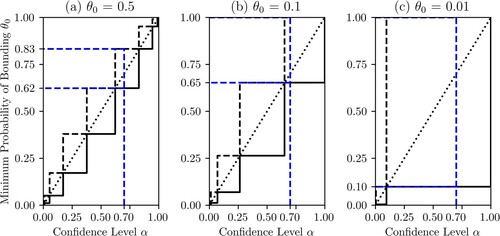
Figure 7. A series of Singh plots used for inference about generated using Equation (13) from
samples of length n = 10 sample with varying degrees of confidence demonstrated by altering the c parameter in Equation (15) (
![]()
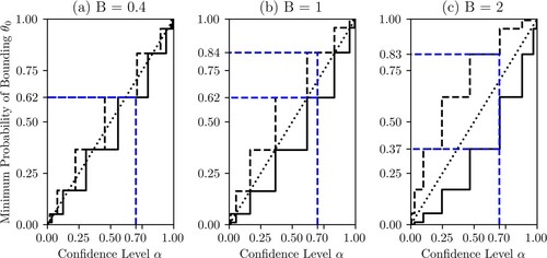
Figure 8. Global Singh plot produced using k = 100 θ values drawn from , each producing
Monte Carlo samples using Equation (13) for inference about θ with a sample size of n = 10 (
![]()
![Figure 8. Global Singh plot produced using k = 100 θ values drawn from [0,1], each producing m=104 Monte Carlo samples using Equation (13) for inference about θ with a sample size of n = 10 (Display full size, SU(α;θ); Display full size, SL(α;θ); Display full size, U(0,1); Display full size, S(α=0.7;θ0)).](/cms/asset/3ae3b3c9-ee52-4f8a-b03e-a20358686bc2/gscs_a_2044814_f0008_oc.jpg)
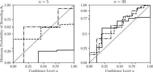
Figure 9. Singh plots representing the coverage probability for a desired α confidence level interval using Equation (Equation19(19)
(19) ) for inference about data generated from Bernoulli distributions with varying θ-parameters. Two plots are shown, for sample sizes of n = 5 (left) and n = 30 (right), each produced from
samples (
![]()