Maximum leave-one-out likelihood method for the location parameter of variance gamma distribution with unbounded density

Figures & data

Figure 1. Plots of full (solid red), LOO (striped blue), LMO (dotted green), and WLOO (dot & striped magenta) log-likelihoods of univariate symmetric VG distribution with $\nu =0.4$ for data set $\{-1,0,1,0\}$ represented by light grey vertical strips. (a) Full and LOO log-likelihoods and (b) LMO and WLOO log-likelihoods.

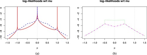
Figure 2. Plot of the full (solid red), LOO (striped blue), LMO (dotted green), and WLOO (dot & striped magenta) log-likelihoods of symmetric VG distribution with $\nu =0.4$ for data set $\{-1,0,1,0,0,1\}$ represented by light grey vertical strips. (a) Full and LOO log-likelihoods and (b) LMO and WLOO log-likelihoods.

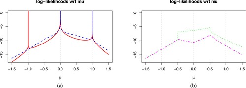
Figure 3. Vioplots to show accuracy of parameter estimates for VG distribution in the first simulation study. The median is displayed as a grey box which is connected by a crimson line. True parameter values represented by the blue lines is drawn for comparison. (a) Vioplot of $\mathit{\mu }$ and (b) Vioplot of $\mathbf{\Sigma }$, $\mathit{\gamma }$, ν.

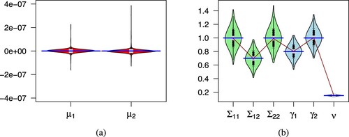
Table 1. ghyp, fixed Δ, adaptive Δ, LOO and WLOO likelihood methods.

Likelihood method	ECM algorithm	Δ
Full ghyp	MCECM	1.2e-4
Full fixed Δ	AECM	1.5e-154
Full adaptive Δ	AECM	adaptive
LOO	ECM/AECM with LPS & line search	1.5e-154
WLOO	ECM with LPS & line search	–

Table 2. Median of 500 accuracy measures of parameter estimates across five likelihood methods with no data multiplicity (R = 1). ‘*’ indicates the methods with lowest absolute error.

Measures	Methods	$\nu =0.05$	$\nu =0.1$	$\nu =0.2$	$\nu =0.5$	$\nu =0.75$	$\nu =1$	$\nu =1.5$
$|\hat{\mathit{\mu }}-\mathit{\mu }|$	Full ghyp	1.2e-10	9.3e-10	7.7e-7	0.0067	0.020	0.031	0.050
	Full fixed Δ	3.5e-28	7.1e-14	6.8e-7	0.0054	0.017	0.030	0.049*
	Full adaptive Δ	3.8e-28	7.7e-14	6.8e-7	0.0036	0.012*	0.026*	0.049*
	LOO	1.6e-28*	1.5e-14*	1.1e-7*	0.0014*	0.012*	0.027	0.050
	WLOO	1.6e-28*	1.5e-14*	1.1e-7*	0.0014*	0.012*	0.027	0.050
$\log \left|\hat{\mathbf{\Sigma }}\right|-\log \left|\mathbf{\Sigma }\right|$	Full ghyp	−3.943	−0.601	−0.038*	−0.016*	0.009*	0.023	−0.013
	Full fixed Δ	−0.103*	0.010*	0.117	0.339	0.472	0.549	−0.012
	Full adaptive Δ	−0.143	−0.059	−0.048	−0.027	−0.010	−0.007	−0.012
	LOO	−0.231	−0.126	−0.074	−0.026	−0.015	−0.009*	−0.011*
	WLOO	−0.232	−0.126	−0.074	−0.026	−0.015	−0.009*	−0.011*
$|\hat{\mathit{\gamma }}-\mathit{\gamma }|$	Full ghyp	0.243	0.060	0.038*	0.038	0.043	0.048	0.059*
	Full fixed Δ	0.048*	0.043	0.038*	0.037	0.039	0.048	0.059*
	Full adaptive Δ	0.048*	0.042*	0.039	0.037	0.038	0.045*	0.059*
	LOO	0.061	0.050	0.041	0.036*	0.038*	0.045*	0.059*
	WLOO	0.061	0.050	0.041	0.036*	0.038*	0.045*	0.059*
$\log \hat{\nu }-\log \nu$	Full ghyp	0.1376	0.0368	0.0067*	−0.0047*	−0.0418	−0.0809	0.0033
	Full fixed Δ	−0.0259	−0.0667	−0.1571	−0.4636	−0.7097	−0.9199	0.0022*
	Full adaptive Δ	0.0052*	0.0055*	0.0091	0.0103	0.0024*	0.0010*	0.0033
	LOO	0.0092	0.0093	0.0110	0.0123	0.0142	0.0090	0.0167
	WLOO	0.0092	0.0093	0.0110	0.0123	0.0142	0.0090	0.0167

Figure 4. Plot of transformed accuracy measures for full ghyp package (red solid line), full fixed Δ (light green striped line), full adaptive Δ (dotted green line), LOO (blue dot & striped line), and WLOO (dash magenta line) likelihoods. The columns from left to right represents the median parameter accuracy measures for $(\hat{\mathit{\mu }},\hat{\mathbf{\Sigma }},\hat{\mathit{\gamma }},\hat{\nu })$ respectively. The rows from top to bottom represents R = 1, 3, 5 respectively where R is the number of times each data point is repeated.

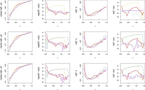
Figure 5. (a) Relative error $\frac{{\widehat{\text{β}}}_{\nu }-{\text{β}}_{\nu }}{{\text{β}}_{\nu }}$ (solid black) against ν. The horizontal solid grey line indicates agreement of ${\widehat{\text{β}}}_{\nu }$ with the proposed optimal rate ${\text{β}}_{\nu }=\frac{1}{2\nu }$. The vertical grey dotted lines represent grid lines for $\nu =\{0,0.2,0.4,0.6,0.8,1\}$. We also include the 95% confidence interval for the relative error (dashed grey). (b) Density of estimates ${\hat{\mu }}_{n,\nu ,1:20,000}$ with its scale standardised using $\mathrm{M}\mathrm{A}\mathrm{D}$ for each ν where n = 100, 000. We use a rainbow colour scheme ranging from red ($\nu =0.02$) to magenta ($\nu =1$).

Figure 6. Kernel density estimates of $\log |{\hat{\mu }}_n|$'s for $\nu =0.02,0.2,0.4,0.6,0.8,1$ and n = 1000 (solid black), 5000 (dashed dark grey), 20, 000 (dotted grey), 100, 000 (dash-dotted light grey) with each n being combined into a single plot for comparison. (a) density plots for $\nu =0.02$ (b) density plots for $\nu =0.2$ (c) density plots for $\nu =0.4$ (d) density plots for $\nu =0.6$ (e) density plots for $\nu =0.8$ and (f) density plots for $\nu =1$.

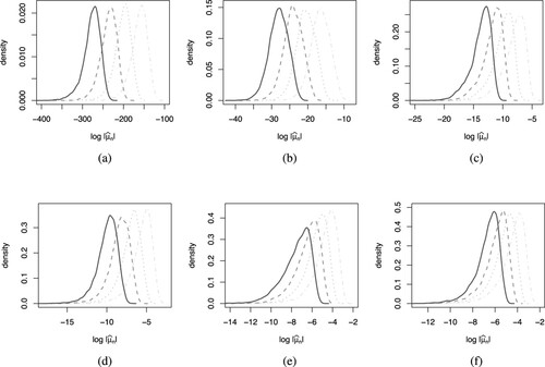
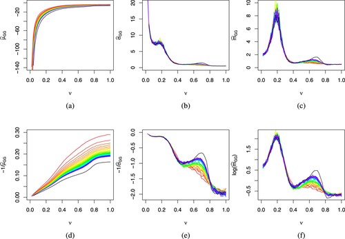
Figure 7. Plot of estimates of generalized Gumbel distribution fitted to the distribution of $\log |{\hat{\mu }}_n|$ against ν. Row 1 plots the $({\hat{\mu }}_{\mathrm{G}\mathrm{G}},{\hat{\sigma }}_{\mathrm{G}\mathrm{G}},{\hat{m}}_{\mathrm{G}\mathrm{G}})$ against ν, respectively, while row 2 plots the transformation $(1/{\hat{\mu }}_{\mathrm{G}\mathrm{G}},-1/{\hat{\sigma }}_{\mathrm{G}\mathrm{G}},\log {\hat{m}}_{\mathrm{G}\mathrm{G}})$ against ν, respectively, to enlarge certain portion of the plots. A rainbow colour scheme ranging from red (n = 500) to magenta (n = 20, 000) is used to denote sample size and the black line represents n = 100, 000. (a) ${\hat{\mu }}_{\mathrm{G}\mathrm{G}}$ vs ν (b) ${\hat{\sigma }}_{\mathrm{G}\mathrm{G}}$ vs ν (c) ${\hat{m}}_{\mathrm{G}\mathrm{G}}$ vs ν (d) $-1/{\hat{\mu }}_{\mathrm{G}\mathrm{G}}$ vs ν (e) $-1/{\hat{\sigma }}_{\mathrm{G}\mathrm{G}}$ vs ν and (f) $\log {\hat{m}}_{\mathrm{G}\mathrm{G}}$ vs ν.