Figures & data
Figure 1. Relationship between cloud-top albedo and cloud optical thickness for different solar zenith angles for a water droplet cloud (mode radius of 10 μm) at a cloud-top height of 4 km, simulated at a wavelength of 760 nm. The cloud optical thickness increases with increasing cloud-top albedo and low solar zenith angles. The increase is less pronounced for high solar zenith angles.
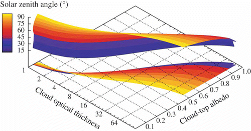
Figure 2. Daily coverage of GOME cloud measurements for 22 May 2002 (a). Errors (as percentage differences) induced in the cloud amount monthly mean averages if the area-weighting is omitted (b).
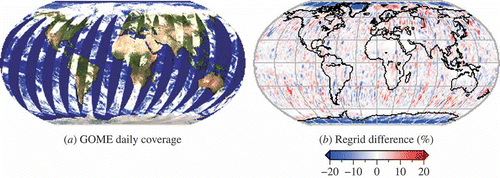
Figure 3. Latitudinal monthly mean (i), zonal mean (ii) and zonal seasonal mean (iii) distributions of the GOME cloud parameters averaged over an 8-year period. (a) Cloud amount (CA), (b) cloud-top pressure (CTP) and (c) cloud optical thickness (COT).
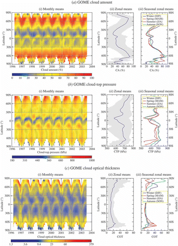
Figure 4. Monthly mean variations of (a) GOME cloud amount, (b) cloud-top pressure and (c) cloud optical thickness in the latitudinal belts 0–15° (red), 15–35° (green), 35–60° (blue). (i) Northern Hemisphere graphs; (ii) Southern Hemisphere part.
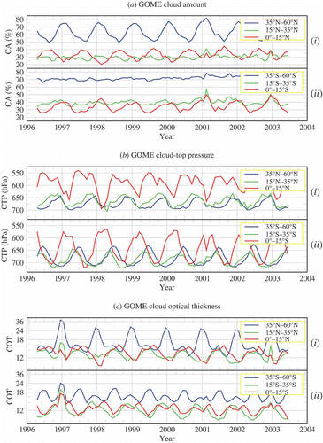
Table 1. Mean values and standard deviations (one sigma) of cloud properties derived from GOME measurements from April 1996 to June 2003. The number of measurements (in millions) used for the calculation of averages is given in parentheses
Figure 5. Average seasonal mean variations of GOME cloud amount (i) and the corresponding standard deviation (ii) from April 1996 to June 2003.
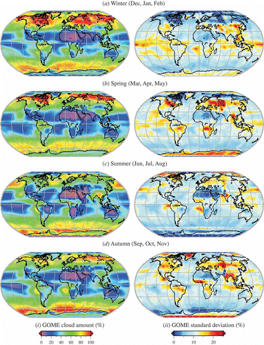
Figure 6. Same as figure 5 but for GOME cloud-top pressure.
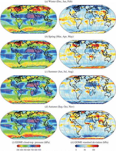
Figure 7. Same as figure 5 but for GOME cloud optical thickness.
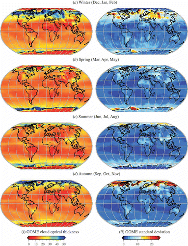
Figure 8. Spatial distribution of 8-year averaged cloud amount (a), cloud-top pressure (b) and cloud-optical thickness (c) as derived from GOME (i) and ISCCP (ii).
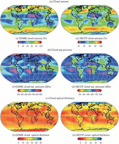
Figure 9. GOME and ISCCP cloud properties deviations (solid lines in blue and red respectively) and trends (dashed lines) averaged over the latitude band 60°N–60°S.
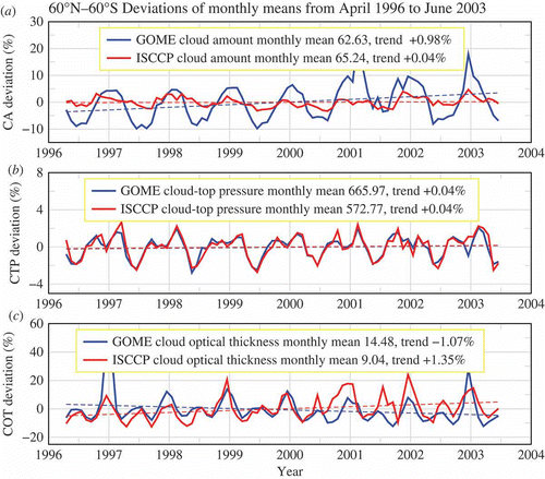
Figure 10. Latitudinal cloud zonal mean variation from April 1996 to June 2003 for GOME in blue, and ISCCP in red. (a) Cloud amount anomaly; (b) cloud-top pressure anomaly and (c) cloud optical thickness anomaly. Global mean values are indicated in the insets. Standard deviations of the GOME (ISCCP) parameters are shown as gray surfaces in the background (dotted red lines in the foreground).
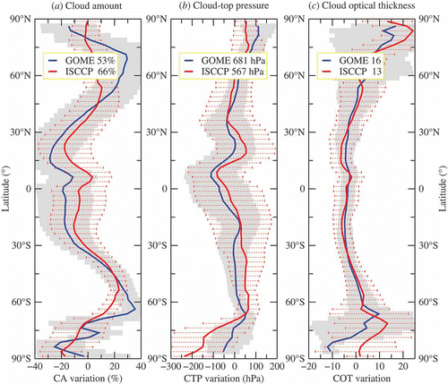
Figure 11. Frequency distribution of (a) cloud amount, (b) cloud-top pressure and (c) cloud optical thickness of GOME global means from April 1996 to June 2003. The normalized histograms are the gray surfaces; the corresponding cumulative histograms are delineated by the black lines.
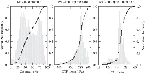
Figure 12. ISCCP D-series cloud types as a function of cloud optical thickness and cloud-top pressure adapted from Stubenrauch (Citation1999c). The approximated range of cloud-top albedo and cloud-top height is given in the top and right axis, respectively. The GOME cloud types do not include optically thin clouds of COT lower than 1.3.
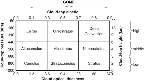
Figure 13. Relative deviation (GOME–ISCCP) between the GOME cloud type distribution and the corresponding ISCCP cloud types using the ISCCP cloud classification method. The relative global occurrence of cloud types and the standard deviation are indicated for each cloud type.
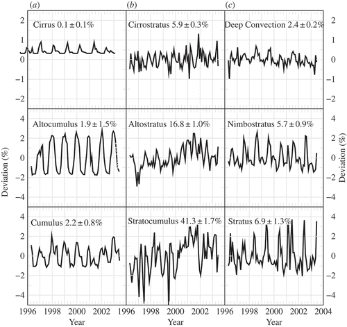
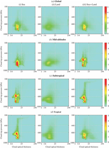
Figure 14. GOME-derived cloud optical thickness and cloud-top pressure variation histograms for different geographical regions: (a) global, (b) mid-latitudes, (c) subtropical and (d) tropical. (i) Sea areas; (ii) land areas; (iii) cumulated sea and land histograms. The global distribution is shown in the first row, followed by results of the mid-latitudes, the subtropical and the tropical zone.