Figures & data
Table 1. Data acquisitions realized during the 2014 growing season. All times are specified in CEST (Central European Summer Time).
Figure 1. Vertical photographs of agricultural crop canopies examined during the 2014 growing season. Phenological status was determined according to the international BBCH scale (Meier Citation2011) and mean chlorophyll contents (Cchl) were derived using a Konica Minolta SPAD-502Plus device.
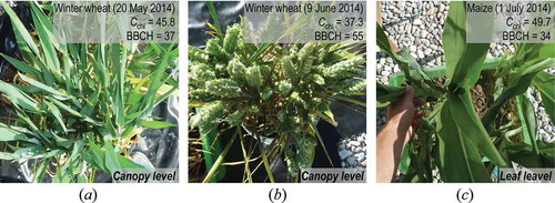
Figure 2. Exemplary presentation of the first (a) and second (b) derivative of a winter wheat canopy reflectance spectrum (instrument: ASD FieldSpec4 standard, acquisition date: 20 May 2014).
Figure 3. Values of gs (mmol m−2 s−1) observed in a winter wheat canopy in May 2014. A vertical trend of increasing gs towards the top layer of the canopy can be observed as well as strong differences between sunlit and shaded areas.
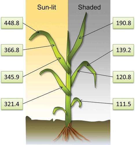
Figure 4. Derived time series of SIF (top) and Ffraction (bottom) derived from the FLD (black solid line with circles) and 3FLD (green dashed line with triangles) methods. Corresponding diurnal trends are indicated by solid lines. The first value of slope and R2 (black) refers to estimates based on the standard FLD approach and the second (green) on 3FLD derived estimates of SIF and Ffraction.
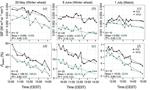
Figure 5. Time series of PRI (black) and S760 (grey). Corresponding diurnal trends are indicated by solid lines. The first value of slope and R2 (black) refers to the PRI and the second (grey) to S760.
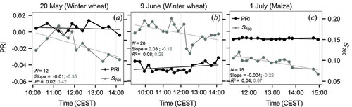
Figure 6. Diurnal variations in stomatal conductance (gs) and Tleaf derived from the SC-1 instrument. Variability of data is indicated by error bars representing one standard deviation.
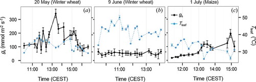
Figure 7. Relationships between 3FLD based SIF and Ffraction retrievals to S760. The individual measurement days are indicated by different colours.
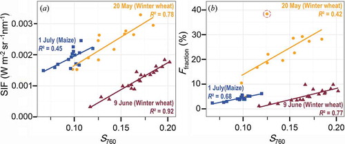
Figure 8. Relationships between 3FLD and FLD derived SIF, S760 and PRI to diurnal measurements of gs. Shaded areas represent the 95% confidence interval. It should be noted that y-axis ranges differ between the three days.
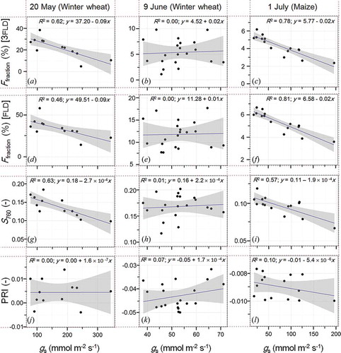
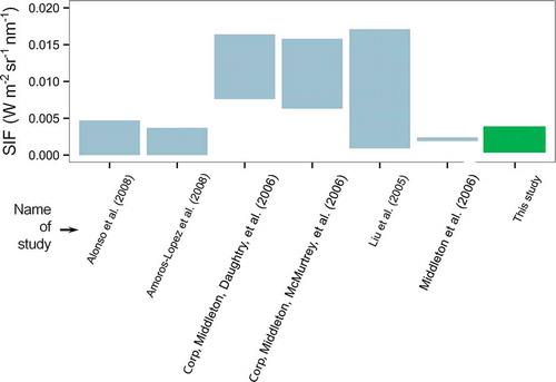
Figure 9. Display of ranges of reported SIF emission values quantified within the O2-A absorption band. Only estimates are displayed, which, comparably to this study, are based on ASD FieldSpec measurements. The value range observed in this study is highlighted in green.