Quantifying suspended sediment concentration in subglacial sediment plumes discharging from two Svalbard tidewater glaciers using Landsat-8 and in situ measurements

Figures & data

Figure 1. Location map of the two Svalbard tidewater glaciers (a) in this study: Kronebreen (b) and Tunabreen (c). Circles represent individual sample locations, with the colour corresponding to the day of sample collection on 2 and 4 May at Kronebreen (green and salmon), and 10, 13, and 14 August at Tunabreen (fuchsia, orange, and yellow, respectively). The red triangles indicate identified subglacial plume discharge locations. Background fjord images are masked Landsat-8 surface reflectance images collected on 2 May 2015 (b) and 14 August 2015 (c).

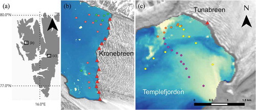
Figure 2. Comparison between Landsat-8 surface reflectance product and in situ field spectrometer reflectance measurements for the red (red diamonds) and red + NIR (black diamonds) spectral ranges at all 44 sample locations. Measure of scatter between the points and the corresponding coloured best-fit line shows the correlation between Landsat-8 surface reflectance product and in situ measurements (r² value of 0.70).

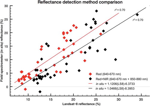
Figure 3. The five Landsat-8 red + NIR surface reflectance images used from Tunabreen (location map, Figure 1(a)), spanning the summer 2015 melt season, showing the subglacial plume discharge location (red triangle), and subglacial sediment plume boundaries (solid red line). These five images from days 187 (a), 190 (b), 213 (c), 226 (d), and 229 (e) are collected between 3 and 23 days apart and highlight the dynamic nature of sediment plumes.

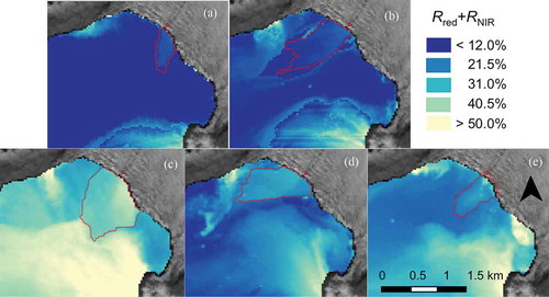
Table 1. Derived equations relating surface reflectance in red and red + NIR wavelengths to SSC at both tidewater glaciers (TWG) and land-terminating glaciers (LTG) in Svalbard and Greenland.

Row	Collection method	SSC range (mg l^−1)	Number of samples	Glacier type, number	SSC (mg)	r^2
1	Landsat-8	0–450	44	2 TWG		0.56
2	Landsat-8	0–450	44	2 TWG		0.65
3	In situ	0–450	44	2 TWG		0.63
4	In situ	0–450	44	2 TWG		0.73
5	Landsat-8	0–200	41	2 TWG		0.55
6	Landsat-8	0–200	41	2 TWG		0.61
7	In situ	0–200	41	2 TWG		0.69
8	In situ	0–200	41	2 TWG		0.75
9	Chu et al. (2009) In situ	0–500	22	1 LTG		0.90
10	Chu et al. (2012) In situ	0–500	25	1 LTG, 1 TWG		0.85
11	Hudson et al. (2014) MODIS	1.20–716	143	3 LTG		0.84

Columns indicate the sensor used to collect the reflectance measurements, the range of SSC values, the number of samples collected, the number of glacier locations and type of glaciers in each calculation, the reflectance equation, and corresponding r² values (columns 2–7, respectively). Rows 1–8 show relationships established in this study, rows 9–11 show the equations derived in other field and remote-sensing studies. It is important to note that Chu et al. (2009), Chu et al. (2012), and Hudson et al. (2014) used the MODIS-equivalent red and NIR wavelength ranges for their calculations, which differs slightly from the Landsat-8 wavelength ranges for the same colours.

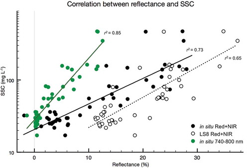
Figure 4. Landsat-8 surface reflectance values (open circles) and in situ field spectrometer reflectance measurements (solid circles) against SSC measurements for all 44 sample locations. The lines represent the best-fit between reflectance and SSC for SSCs in the 0–450 mg l⁻¹ range (all 44 samples) and 0–200 mg l⁻¹ range (41 samples) and for in situ and satellite reflectance sampling methods, in the red band range (left) and red + NIR band range (right). Legends correspond to both plots.

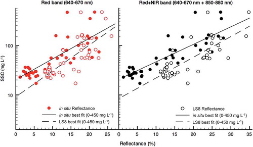
Table 2. Plume area (m²), calculated surface sediment load (kg), and constructed 6 days PDD value (°C) for each ice- and cloud-free image during the summer 2015 melt season at Kronebreen and Tunabreen glaciers.

DOY	Glacier	Plume area (m^2)	Surface sediment load (kg)	6 days PDD (°C)	r^2 (p-value)
122	Kronebreen	1289,700	1151.60	–	–
124	Kronebreen	1649,700	1216.96	–	–
147	Kronebreen	140,400	904.97	–	–
152	Kronebreen	22,500	354.34	–	–
172	Kronebreen	407,700	318.88	25.40	0.89 (p < 5 × 10^−^3)
186	Kronebreen	1102,500	1134.12	28.30
190	Kronebreen	1394,100	3203.07	39.70
213	Kronebreen	6617,700	8765.42	53.10
220	Kronebreen	3326,400	3695.43	40.00
225	Kronebreen	2628,000	2573.81	40.80
187	Tunabreen	180,000	112.54	39.10	0.94 (p < 6 × 10^−^3)
190	Tunabreen	537,300	290.88	49.50
213	Tunabreen	841,500	13,774.97	64.50
226	Tunabreen	558,900	1682.94	53.60
229	Tunabreen	322,200	1009.50	51.60

The correlation between surface sediment load and constructed 6 days PPD values (r² value) as well as significance (p-value) are shown for Kronebreen and Tunabreen glaciers. Each calculation includes only points with both a surface sediment load value and a constructed 6 days PDD value.

Figure 5. Plot showing the constructed 6 days PDD sum prior to the data point (solid black line) over the 2015 melt season at Tunabreen (top) and Kronebreen (bottom), with the dashed black lines indicating the days of Landsat-8 imagery, and the red dotted lines indicating the start and end of the plume viewing period; the start being the first image with an ice-free terminus and the end being the first image with a solar zenith angle too high to calculate surface reflectance. The total surface sediment load for each of the Landsat-8 images is shown as green dots.

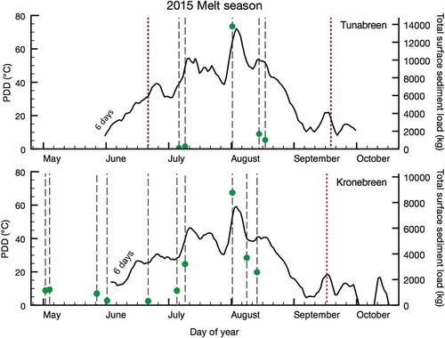
Figure 6. Average spectral profile (purple line) collected in a subglacial plume at Templefjorden. Filled curves represent the Landsat-8 spectral range and weighting function for the blue, green, red, and NIR bands (from left to right), while the dashed line represents the optimal range for SSC detection (740–800 nm), and the bracket indicating the wavelength gap between the red and NIR bands.

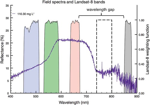
Figure 7. SSC versus surface reflectance in 740–800 nm (green circles, 740–800 nm) plotted along side the models (from Figure 4) with the highest r² value relationships collected from the field spectrometer (red + NIR, black circles) and the Landsat-8 surface reflectance product (red + NIR, open circles). We recommend the spectral range 740–800 nm be considered for inclusion in the next space mission.

Chu, V. W., L. C. Smith, A. K. Rennermalm, R. R. Forster, J. E. Box, and N. Reeh. 2009. “Sediment Plume Response to Surface Melting and Supraglacial Lake Drainages on the Greenland Ice Sheet.” Journal of Glaciology 55 (194): 1072–1082. doi:10.3189/002214309790794904.

 Web of Science ®Google Scholar

Chu, V. W., L. C. Smith, A. K. Rennermalm, R. R. Forster, and J. E. Box. 2012. “Hydrologic Controls on Coastal Suspended Sediment Plumes around the Greenland Ice Sheet.” The Cryosphere 6 (1): 1–19. doi:10.5194/tc-6-1-2012.

 Web of Science ®Google Scholar

Hudson, B., I. Overeem, D. McGrath, J. P. M. Syvitski, A. Mikkelsen, and B. Hasholt. 2014. “MODIS Observed Increase in Duration and Spatial Extent of Sediment Plumes in Greenland Fjords.” The Cryosphere 8: 1161–1176. doi:10.5194/tc-8-1161-2014.

 Web of Science ®Google Scholar