Synthetic retrieval of hourly net ecosystem exchange using the neural network model with combined MI and GOCI geostationary sensor datasets and ground-based measurements

Figures & data

Table 1. Detailed characteristics of the COMS MI and GOCI sensors, which collected the data used as input variables for the NN model.

Satellite sensor (Orbit type)	Wavelength (nm)	Spatial resolution
MI	Visible: 550–800 shortwave infrared: 3500–4000 Water vapor: 6500–7000 Infrared 1: 10,300–11,300 Infrared 2: 11,500–15,500	1000 m (4000 m) at nadir visible (infrared)
GOCI	Band1 402–422 Band2 433–453 Band3 480–500 Band4 545–565 Band5 650–670 Band6 675–685 Band7 735–755 Band8 845–885	500 m in the South Korea region

Figure 1. Location of the CO₂ flux tower site (marked with white rectangle) for the eddy covariance measurements on Mt. Halla, Jeju Island, South Korea (Image source from Daum map service through QGIS).

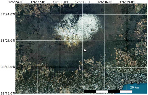
Figure 2. Scatter plots of net ecosystem carbon dioxide (CO₂) exchange (NEE) derived from eddy covariance measurements compared with the results of the neural network (NN) model estimations based on combined satellite imagery with ground measurements during daytime. (a) Bowen ratio, (b) net solar radiation, Rn, (c) Bowen Ratio and Rn, (d) Meteorological Imager, MI channel, (e) Geostationary Ocean Color Imager, GOCI, (f) MI and GOCI, (g) MI, GOCI, Bowen Ratio, and Rn, (h) MI, GOCI, Sensible heat and Latent and Rn. The black line is the reference line. Bowen, Rn, Sensible, and Latent represent the Bowen ratio, net radiation, sensible heat, and latent heat flux, respectively.

Figure 3. Scatter plots of net ecosystem carbon dioxide (CO₂) exchange (NEE) derived from eddy covariance measurements compared with the results of the neural network (NN) model estimations based on combined satellite imagery with ground measurements during night-time. (a) Bowen ratio, (b) net solar radiation, Rn, (c) Bowen Ratio and Rn, (d) Meteorological Imager, MI channel, (e) Geostationary Ocean Color Imager, GOCI, (f) MI and GOCI, (g) MI, GOCI, Bowen Ratio, and Rn, (h) MI, GOCI, Sensible heat and Latent and Rn. The black line is the reference line. Bowen, Rn, Sensible, and Latent represent the Bowen ratio, net radiation, sensible heat, and latent heat flux, respectively.

Figure 4. Plots of the eigenvalues (in closed dots) and cumulative percentage eigenvalues (in opened dots) according to the principal component number for the daytime (left panels) and night-time (right panels) for: (a, b): combined satellites Meteorological Imager (MI) and Geostationary Ocean Color Imager (GOCI) input data, (c, d): All variables including the ground-based measurements. Each vertical dashed line represents the final principal component number that satisfies the cumulative percentage of eigenvalues of at least 99%.

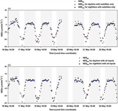
Figure 5. Temporal variations in NEE based on the NN simulation model from the test data set (16–23 May) using (a) satellite data (MI and GOCI) as the input variables and (b) all inputs including ground measurements. The red dots represent daytime NEE, and the blue dots represent night-time NEE. The seven light grey areas from 5 p.m. until 8 a.m. represent the night-time period.