Figures & data
Figure 1. SST (shaded colour) blended with multi-satellite images and AVISO surface current anomalies (arrows) on 28 September 2014. The thicker black contour and the thinner white lines indicate the periphery of the automatically identified cold dome and isobaths, respectively. The dotted blue line represents the ground track of the satellite altimeter (Track 240) crossing precisely over the cold dome.
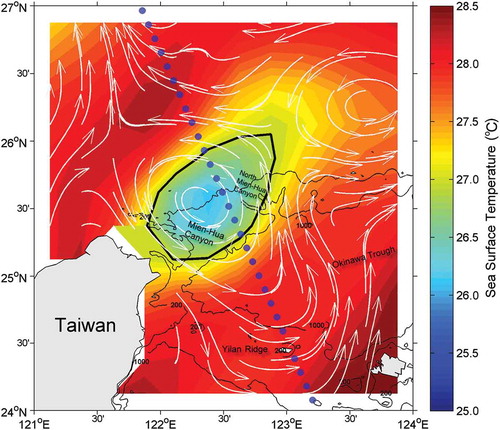
Figure 2. Empirical orthogonal function (EOF) of mode 1 (54%) with along-track SLA (track 240): (a) eigenvector of mode 1 (EV1) and (b) principal component of mode 1 (PC1). (c) Wavelet power spectrum of PC1 using the Morlet wavelet. The black contour encloses significant regions (90% confidence level); a lighter shade indicates the cone of influence where edge effects might distort the diagram.
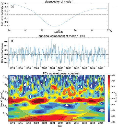
Figure 3. EOF of mode 1 (45%) with SST: (a) EV1 and (b) PC1.
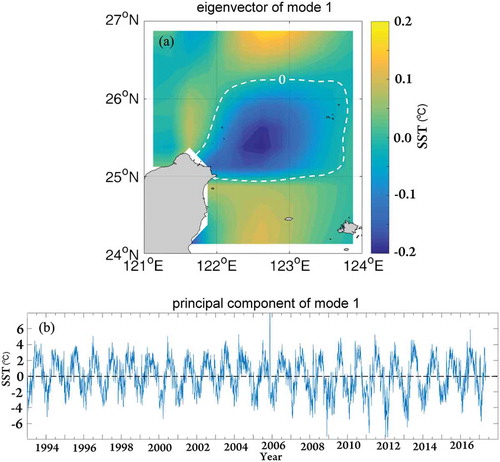
Figure 4. Twelve-month low-pass filtered time series of (a) SLA PC1 (blue) and SST PC1 (orange) and (b) ONI (yellow) and PDO (green).
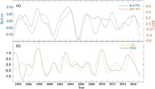
Figure 5. Lagged correlations of SLA PC1 with SST PC1, ONI, and PDO. Dash-dots indicate an insignificant correlation coefficient (r) at the 95% confidence level.
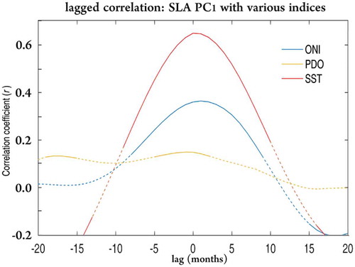
Figure 6. Wind fields (arrows) and wind stress curl (shaded) for (a) SLA PC1 > 0 and for (b) SLA PC1 < 0.
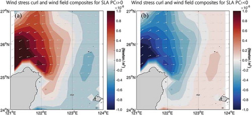
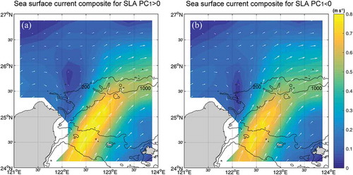
Figure 7. Surface current vectors (arrows) and speed (shaded) derived from ADT for (a) SLA PC1 > 0 and for (b) SLA PC1 < 0.