Implementation of machine-learning classification in remote sensing: an applied review

Figures & data

Table 1. R packages used by caret.

Algorithm	Package	Citation
RF	Ranger	Wright (2017)
SVM	Kernlab	Karatzoglou, Smola, and Hornik (2016)
DT	Rpart	Therneau, Atkinson, and Ripley (2017)
Boosted DT	C50	Kuhn et al. (2015)
ANN	Nnet	Ripley and Venables (2016)
k-NN	Caret	Kuhn et al. (2016)

Table 2. Number of samples for Indian pines data.

Class	Number of pixels
	Training	Validation	Total
Alfalfa	14	40	54
Corn	626	1876	2502
Grass	131	392	523
Hay	122	367	489
Oats	5	15	20
Soybeans	1012	3038	4050
Trees	324	970	1294
Wheat	53	159	212
Total	2287	6857	9144

Figure 1. Indian Pines AVIRIS hyperspectral data and classification results. The image was acquired 12 June 1992. The centre of the image is at approximately 40.46111° N, 87.01111° W, and the image is oriented with North up. (a) False colour composite of blue = band 28, green = band 65, and red = band 128. (b) The reference class map. (c) The SVM classification using a balanced training data set and feature selection. (d) The RF classification using a balanced training data set and feature selection.

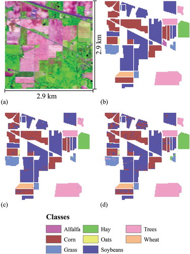
Table 3. Number of samples for urban GEOBIA data.

Class	Number of pixels
	Training	Validation	Total
Asphalt	14	45	59
Building	25	97	122
Car	15	21	36
Concrete	23	93	116
Grass	29	83	112
Pool	15	14	29
Shadow	16	45	61
Soil	14	20	34
Tree	17	89	106
Total	168	507	675

Table 4. Classification results for Indian pines data.

Preprocessing	Accuracy measure	SVM	DT	RF	Boosted DT	ANN	k-NN
None	Overall accuracy (%)	89.1	78.3	87.1	87.2	85.1	78.6
	Kappa	0.844	0.687	0.814	0.817	0.787	0.686
Feature selection (A)	Overall accuracy (%)	94.2	78.3	88.0	88.3	91.0	88.0
	Kappa	0.918	0.687	0.827	0.832	0.871	0.829
Feature selection (B)	Overall accuracy (%)	86.1	77.2	83.4	83.0	86.3	84.1
	Kappa	0.801	0.672	0.761	0.758	0.803	0.772
Balanced training data	Overall accuracy (%)	89.5	65.8	87.4	87.0	43.0	76.3
	Kappa	0.850	0.541	0.820	0.814	0.269	0.666
Feature selection (A) +  balanced training data	Overall accuracy (%)	94.4	65.8	87.8	87.6	85.9	87.3
	Kappa	0.921	0.542	0.826	0.823	0.802	0.820
Feature selection (B) +  balanced training data	Overall accuracy (%)	86.6	71.2	83.8	83.2	83.3	82.1
	Kappa	0.810	0.594	0.768	0.760	0.763	0.748

Table 5. Classification results for urban GEOBIA data.

Preprocessing	Accuracy measure	SVM	DT	RF	Boosted DT	ANN	k-NN
None	Overall accuracy (%)	76.3	68.1	81.5	76.9	67.5	72.4
	Kappa	0.724	0.629	0.782	0.733	0.621	0.677
Feature selection (A)	Overall accuracy (%)	76.9	68.8	81.7	77.3	71.4	75.0
	Kappa	0.730	0.636	0.785	0.735	0.668	0.706
Feature selection (B)	Overall accuracy (%)	77.1	68.1	78.3	75.0	72.8	72.8
	Kappa	0.732	0.627	0.746	0.708	0.683	0.682
Balanced training data	Overall accuracy (%)	76.1	69.0	80.5	81.9	70.8	68.4
	Kappa	0.722	0.641	0.771	0.788	0.661	0.636
Feature selection (A) +  balanced training data	Overall accuracy (%)	75.4	70.0	81.3	75.5	72.0	67.1
	Kappa	0.713	0.652	0.781	0.715	0.674	0.620
Feature selection (B) +  balanced training data	Overall accuracy (%)	75.2	71.0	76.1	74.0	73.6	64.7
	Kappa	0.709	0.664	0.722	0.696	0.692	0.589

Table 6. Classification of Indian pines data using RF and original training data.

		Reference
		Alfalfa	Corn	Grass	Hay	Oats	Soybeans	Trees	Wheat	Total	User’s accuracy
	Alfalfa	17	0	1	1	0	0	0	0	19	0.90
	Corn	0	1356	2	0	2	233	0	1	1594	0.85
	Grass	1	2	321	7	0	4	2	0	337	0.95
Prediction	Hay	17	0	27	359	0	4	0	0	407	0.88
	Oats	0	0	0	0	4	0	0	0	4	1.00
	Soybeans	5	518	19	0	5	2795	1	1	3344	0.84
	Trees	0	0	22	0	0	1	967	4	994	0.97
	Wheat	0	0	0	0	4	1	0	153	158	0.97
	Total	40	1876	392	367	15	3038	970	159
	Producer’s accuracy	0.43	0.72	0.83	0.98	0.27	0.92	1.00	0.96

Overall accuracy is 87.1%.

Table 7. Classification of Indian pines data using RF and balanced training data.

		Reference
		Alfalfa	Corn	Grass	Hay	Oats	Soybeans	Trees	Wheat	Total	User’s accuracy
	Alfalfa	18	2	3	2	0	2	0	0	27	0.67
	Corn	0	1442	1	0	1	289	0	1	1734	0.83
	Grass	1	3	328	4	3	14	7	0	360	0.91
Prediction	Hay	17	2	26	361	0	6	0	0	412	0.88
	Oats	0	0	0	0	7	0	0	0	7	1.00
	Soybeans	4	427	9	0	1	2723	0	1	3165	0.86
	Trees	0	0	25	0	1	2	963	6	997	0.97
	Wheat	0	0	0	0	2	2	0	151	155	0.97
	Total	40	1876	392	367	15	3038	970	159
	Producer’s accuracy	0.45	0.77	0.84	0.98	0.47	0.90	0.99	0.95

Overall accuracy is 87.4%.

Table 8. Classification of Indian pines data using SVM and original training data.

		Reference
		Alfalfa	Corn	Grass	Hay	Oats	Soybeans	Trees	Wheat	Total	User’s accuracy
	Alfalfa	23	1	1	7	0	0	0	0	32	0.72
	Corn	0	1498	0	0	3	260	0	0	1761	0.85
	Grass	0	1	347	4	1	8	7	0	368	0.94
Prediction	Hay	13	0	14	355	0	1	0	0	383	0.93
	Oats	0	1	0	0	6	1	0	1	9	0.67
	Soybeans	4	374	23	1	1	2767	1	1	3172	0.87
	Trees	0	1	7	0	0	1	960	2	971	0.99
	Wheat	0	0	0	0	4	0	2	155	161	0.96
	Total	40	1876	392	367	15	3038	970	159
	Producer’s accuracy	0.58	0.80	0.89	0.97	0.40	0.91	0.99	0.98

Overall accuracy is 89.1%.

Table 9. Classification of Indian pines data using SVM and balanced training data.

		Reference
		Alfalfa	Corn	Grass	Hay	Oats	Soybeans	Trees	Wheat	Total	User’s accuracy
	Alfalfa	24	2	2	6	0	0	0	0	34	0.71
	Corn	0	1558	0	0	3	300	0	0	1861	0.84
	Grass	0	1	348	4	1	8	8	0	370	0.94
Prediction	Hay	12	0	14	357	0	1	0	0	384	0.93
	Oats	0	1	0	0	6	1	0	1	9	0.67
	Soybeans	4	313	21	0	1	2727	1	1	3068	0.89
	Trees	0	1	7	0	0	1	959	2	970	0.99
	Wheat	0	0	0	0	4	0	2	155	161	0.96
	Total	40	1876	392	367	15	3038	970	159
	Producer’s accuracy	0.60	0.83	0.89	0.97	0.40	0.90	0.99	0.98

Overall accuracy is 89.1%.

Table 10. User-defined parameter examples.

Algorithm	User-defined parameters	Example references
k-Nearest neighbour	Number of neighbours considered (k)	Cover and Hart (1967), Dudani (1976), Bailey and Jain (1978)
MLP artificial neural networks with backpropagation	Activation function Number of hidden layers Number of nodes in each layer Learning rate Momentum factor Weight initialization Number of iterations	Rumelhart and McClelland (1986)
Decision trees	Pruning parameters (cp)	Quinlan (1986)
Boosted decision trees (Adaboost method)	Number of iterations or trees (n)	Freund and Schapire (1996)
Random forests	Number of trees (n) Number of variables randomly sampled as candidates at each split (m)	Breiman (2001)
Support vector machines using polynomial kernel	Cost or slack parameter (C) Kernel type Kernel-dependent parameters: Polynomial: polynomial order (p) Radial basis: gamma (γ)	Cortes and Vapnik (1995), Vapnik (1995)

MLP: Multilayer perception.

Figure 2. Impact of parameters on classification performance evaluated by comparison against validation data. Note that the y-axis scaling for (c) and (d) differ from that of the other graphs.

(a) GEOBIA k–NN, (b) Indian pines k–NN, (c) GEOBIA DT, (d) Indian pines DT, (e) GEOBIA RF, (f) Indian pines RF, (g) GEPBIA SVM, (h) Indian pines SVM.

Table 11. Training/Tuning and prediction times.

Classification task	Algorithm
	SVM	DT	RF	Boosted DT	ANN	k-NN
Urban GEOBIA training time (ms)	175.7	147.4	324.5	287.9	398.3	126.8
Urban GEOBIA training and tuning time (s)	7.5	1.2	53.1	62.7	59.2	1.2
Urban GEOBIA predicting time (ms)	83.7	18.1	176.3	272.3	23.2	24.8
Indian Pines training time (ms)	2020.9	411.3	1935.2	109,004.7	1817.4	209.8
Indian Pines training and tuning time (s)	169.3	5.5	509.3	2334.7	304.6	20.0
Indian Pines predicting time (ms)	2388.2	188.2	584.1	5814.6	201.6	3523.6

Table 12. Software implementation of machine learning.

Software	Algorithm
	k-NN	ANNs	DTs^1	Boosted DTs	RF	SVM
Geospatial software
ArcGIS 10.5/ArcPro 2					X	X
eCognition Developer 9	X		X		X	X
ENVI 5.4		X				X
Erdas Imagine 2016
TerrSet/IDRISI 18.3	X	X	X
QGIS 2.18	X	X	X	X	X	X
Other software
Matlab 9.3	X	X	X	X	X	X
R 3.4	X	X	X	X	X	X
Python scikit-learn 0.19.1	X	X	X	X	X	X
Weka 3.9	X	X	X	X	X	X

¹We define DTs as algorithms that generate a decision tree using machine learning. Our definition excludes expert-system decision trees, where the trees are developed from expert knowledge. Both ENVI 5.4 and Imagine 2016 have environments for encoding expert systems.

ArcGIS is sold by ESRI (Redlands, CA, USA), eCogntion by Trimble (Sunnyvale, CA, USA), ENVI by Harris Geospatial Solutions (Melbourne, FL, USA), and TerrSet/IDRISI by Clark Labs (Worcester, MA, USA). Matlab is sold by MathWorks (Natick, MA, USA). QGIS, R, scikit-learn, and Weka are open source software. QGIS, R, and scikit-learn are collaborative efforts; Weka is produced by the Machine Learning Group at the University of Waikato, New Zealand.

Wright, M. N. 2017. “Ranger: A Fast Implementation of Random Forests.” R package version 0.8.0. https://cran.r-project.org/web/packages/ranger/index.html.

 Google Scholar

Karatzoglou, A., A. Smola, and K. Hornik. 2016. “Kernlab: Kernel-Based Machine Learning Lab.” R package version 0.9-25. https://cran.r-project.org/web/packages/kernlab/index.html.

 Google Scholar

Therneau, T., B. Atkinson, and B. Ripley. 2017. “Rpart: Recursive Partitioning and Regression Trees.” R package version 4.1-11. https://cran.r-project.org/web/packages/rpart/index.html.

 Google Scholar

Kuhn, M., S. Weston, N. Coulter, M. Culp, and R. Quinlan. 2015. “C50: C5.0 Decision Trees and Rule-Based Models.” R package version 0.8.0. https://cran.r-project.org/web/packages/C50/index.html.

 Google Scholar

Ripley, B., and W. Venables. 2016. “nnet: Feed-Forward Neural Networks and Multinomial Log-Linear Models.” R package version 7.3-12. https://cran.r-project.org/web/packages/nnet/index.html.

 Google Scholar

Kuhn, M., J. Wing, S. Weston, A. Williams, C. Keefer, A. Engelhardt, T. Cooper, et al. 2016. “Caret: Classification and Regression Training.” R package version 6.0-73. https://cran.r-project.org/web/packages/caret/index.html.

 Google Scholar

Cover, T. M., and P. E. Hart. 1967. “Nearest Neighbor Pattern Classification.” IEEE Transactions on Information Theory 13: 21–27. doi:10.1109/TIT.1967.1053964.

 Web of Science ®Google Scholar

Dudani, S. A. 1976. “The Distance-Weighted K-Nearest Neighbor Rule.” IEEE Transactions on Systems, Man, and Cybernetics SMC, no. 6: 325–327. doi:10.1109/TSMC.1976.5408784.

 Web of Science ®Google Scholar

Bailey, T., and A. K. Jain. 1978. “A Note on Distance-Weighted K-Nearest Neighbor Rules.” IEEE Transactions on Systems, Man, and Cybernetics SMC, 8 (4): 311–313.

 Web of Science ®Google Scholar

Rumelhart, D. E., and J. L. McClelland. P. D. P. Research Group. 1986. Parallel Distribution Processing: Explorations in the Microstructure of Cognition. London, UK: MIT Press.

 Google Scholar

Quinlan, J. R. 1986. “Induction of Decision Trees.” Machine Learning 1: 81–106. doi:10.1007/BF00116251.

 Google Scholar

Freund, Y., and R. E. Schapire. 1996. “Experiments with the New Boosting Algorithm.” Thirteenth International Conference on Machine Learning 96: 148–156.

 Google Scholar

Breiman, L. 2001. “Random Forests.” Machine Learning 54 (1): 5–32. doi:10.1023/A:1010933404324.

 Web of Science ®Google Scholar

Cortes, C., and V. Vapnik. 1995. “Support-Vector Networks.” Machine Learning 20: 273–297. doi:10.1007/BF00994018.

 Web of Science ®Google Scholar