Aboveground forest biomass derived using multiple dates of WorldView-2 stereo-imagery: quantifying the improvement in estimation accuracy

Figures & data

Figure 1. Location of the study area and sample plots in southern Finland. The total number of sample plots (n = 364) is comprised of 91 sample plot clusters.

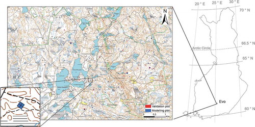
Figure 2. Workflow for obtaining four different aboveground biomass (AGB) estimates for year 2016. Area-based approach (ABA) was used to predict AGB for each plot in 2014 (AGB₂₀₁₄) and (a) 2016 (AGB₂₀₁₆). Then (b) AGB₂₀₁₄ estimates were growth projected to 2016 (AGB_{Projected_2016}) and (c) combined with AGB₂₀₁₆ (AGB_{Combined_2016}). (d) AGB prediction model developed with 2014 data was also applied to 2016 data (AGB_{2016_pred2014}). Accuracies of AGB₂₀₁₆, AGB_{Projected_2016}, AGB_{Combined_2016}, and AGB_{2016_pred2014} were validated at sample plot level.

Table 1. The descriptive statistics of the aboveground biomass (AGB, Mg ha⁻¹) variation within the modelling and validation sample plots in 2014 and 2016.

Sample plot set	Year	n	Minimum	Mean	Maximum	Standard deviation
Modelling	2014	248	11.6	132.5	312.1	54.5
Validation	2014	84	39.2	137.0	238.5	50.6
Modelling	2016	204	12.7	138.4	311.5	54.3
Validation	2016	84	42.3	141.3	242.2	53.3

Table 2. Parameters of the used WorldView-2 image pairs.

Image	11 July 2014 (1)	11 July 2014 (2)	13 September 2016 (1)	13 September 2016 (2)
Mean in-track angle (°)	0.5	−11.6	9.1	−8.8
Mean cross-track angle (°)	−6.8	−7.1	11.1	10.5
Mean off-nadir angle (°)	6.8	13.6	14.3	13.7

Table 3. Features extracted from the normalized digital surface model derived from WorldView-2 image-based point clouds and feature definitions.

Feature category	Feature	Definition
Tree height	Hmax	Maximum of the normalized heights of all points
	Hmean	Arithmetic mean of normalized heights of all points above 2 m height threshold
	Hmod	Mode of normalized heights of all points above 2 m height threshold
	H10–H90	10% to 90% percentiles of normalized heights of all points above 2 m height threshold with a 10% increment
Canopy cover	P	NH≤ 2/Ntotal × 100, where Ntotal is the number of all points and NH≤ 2 the number of points below and equal to 2 m height threshold
	C1–C10	Ci = Ni/Ntotal, where i = 1 to 10, Ni is the number of points within ith layer when tree height was divided into 10 intervals starting from 2 m height, Ntotal is the number of all points
Variation in tree heights	Hstd	Standard deviation of normalized heights of all points above 2 m threshold
	Hcv	Coefficient of variation calculated as Hstd/Hmean

Figure 3. (a) 90th height percentile (H₉₀), (b) penetration percentage (P), and (c) standard deviation of height (H_std) derived from WorldView-2 data for years 2014 and 2016.

Table 4. Accuracy of the predicted aboveground biomass (AGB) estimates in validation sample plots (n = 84) in 2014.

k	Bias (mg ha^−1)	Bias (%)	RMSE (mg ha^−1)	RMSE (%)	Standard deviation (mg ha^−1)
1	−3.7	−2.7	36.7	26.8	52.7
3	−7.0	−5.1	32.4	23.6	48.1
5	−6.7	−4.9	31.5	23.0	46.9
7	−6.1	−4.4	28.9	21.1	45.8
9	−7.7	−5.6	30.2	21.9	45.7

Table 5. Accuracy of the predicted aboveground biomass (AGB) estimates in validation sample plots (n = 84) in 2016.

k	Bias (mg ha^−1)	Bias (%)	RMSE (mg ha^−1)	RMSE (%)	Standard deviation (mg ha^−1)
1	−14.2	−10.0	49.5	35.0	64.8
3	−12.9	−9.1	37.9	26.9	53.6
5	−10.6	−7.5	36.7	26.0	50.6
7	−11.6	−8.2	37.0	26.2	49.5
9	−12.3	−8.7	36.9	26.1	50.3

Figure 4. (a) Aboveground biomass prediction for 2014 (AGB₂₀₁₄) and 2016 (AGB₂₀₁₆) and (b) respective estimation errors at sample plot level.

Figure 5. Aboveground biomass map for (a) 2014 (AGB₂₀₁₄) and (b) 2016 (AGB₂₀₁₆) as well as (c) growth-projected aboveground biomass (AGB_{Projected_2016}) and (d) combined aboveground biomass (AGB_{Combined_2016}) maps covering the study area (61.19°N, 25.11°E). AGB_{Projected_2016} and AGB_{Combined_2016} maps should only be used for undisturbed areas.

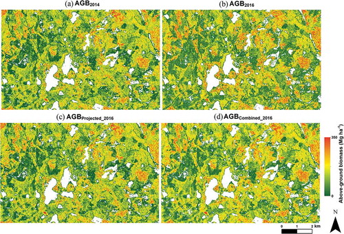
Table 6. Accuracy of the predicted aboveground biomass estimates (AGB₂₀₁₆), projected AGB estimates (AGB_{Projected_2016}), combined AGB estimates (AGB_{Combined_2016}), and estimates predicted using model from year 2014 (AGB_{2016_pred2014}) in validation sample plots (n = 84) in 2016. AGB_{Combined_2016} is obtained by averaging AGB₂₀₁₆ and AGB_{Projected_2016} at the sample plot level.

	Bias (mg ha^−1)	Bias (%)	RMSE (mg ha^−1)	RMSE (%)	Standard deviation (Mg ha^−1)
AGB2016	−10.6	−7.5	36.7	26.0	50.6
AGBProjected_2016	9.9	7.0	30.8	21.8	44.4
AGBCombined_2016	−0.4	−0.3	29.5	20.9	45.7
AGB2016_pred2014	−27.7	−19.6	46.9	33.2	49.4

Figure 6. Variation in relative RMSE when projected inventory (AGB_{Projected_2016}) is combined with recent inventory (AGB₂₀₁₆) with varying weights. Weight ‘0.1’ means that combined estimate is calculated by giving weight of ‘0.1’ for AGB_{Projected_2016} and ‘0.9’ to AGB_2016.