
Figures & data
Figure 1. The islands and complexes within the Florida Key deer range and the Lower Keys marsh rabbits range. Key deer inhabit 20–25 islands within the boundaries of National Key Deer Refuge (Lopez et al. Citation2004) and the majority are found throughout 11 islands and complexes in the Lower Florida Keys from Sugarloaf Key (west) to Big Pine Key (east; Harveson et al. Citation2006). About 75% of the total Key deer herd reside on Big Pine (2,548 ha) and No Name (461 ha) Keys (Lopez et al. Citation2004). Marsh rabbits occupy only a few of the larger islands in the Lower Florida Keys, including Boca Chica, Saddlebunch, Sugarloaf, Little Pine, and Big Pine Keys; and smaller islands surrounding those larger islands (United States Fish and Wildlife Service [USFWS] Citation2019). The inset map, marked as A, indicates the location of the study area
![Figure 1. The islands and complexes within the Florida Key deer range and the Lower Keys marsh rabbits range. Key deer inhabit 20–25 islands within the boundaries of National Key Deer Refuge (Lopez et al. Citation2004) and the majority are found throughout 11 islands and complexes in the Lower Florida Keys from Sugarloaf Key (west) to Big Pine Key (east; Harveson et al. Citation2006). About 75% of the total Key deer herd reside on Big Pine (2,548 ha) and No Name (461 ha) Keys (Lopez et al. Citation2004). Marsh rabbits occupy only a few of the larger islands in the Lower Florida Keys, including Boca Chica, Saddlebunch, Sugarloaf, Little Pine, and Big Pine Keys; and smaller islands surrounding those larger islands (United States Fish and Wildlife Service [USFWS] Citation2019). The inset map, marked as A, indicates the location of the study area](/cms/asset/fcc22567-517a-41d7-a9c6-91ac864fab8e/tres_a_1800125_f0001_c.jpg)
Figure 2. Different vegetation types appear as the response to the changing elevation (figure taken from Lopez et al. Citation2004). Developed areas usually occur between mangrove and buttonwood (Lopez et al. Citation2004)
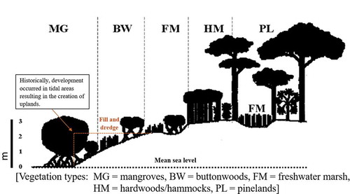
Figure 3. Red mangrove in the Lower Florida Keys (Lopez Citation2001)
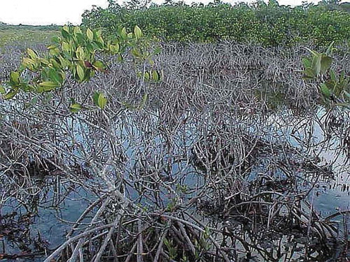
Figure 4. The zonation of 3 different mangroves with respect to elevation
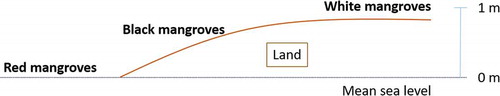
Figure 5. Buttonwood occurring in the Lower Florida Keys (Lopez Citation2001)
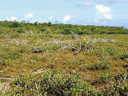
Figure 6. Freshwater marsh occurring in the Lower Florida Keys (Lopez Citation2001)
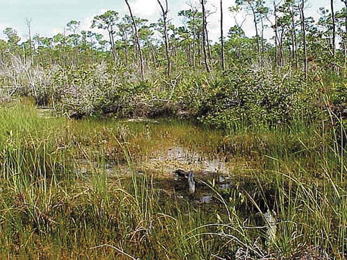
Figure 7. Hammocks occurring in the Lower Florida Keys (Lopez Citation2001)
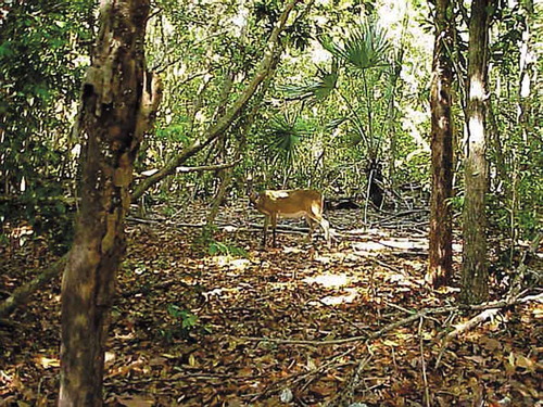
Figure 8. Pinelands occurring in the Lower Florida Keys (Lopez Citation2001)
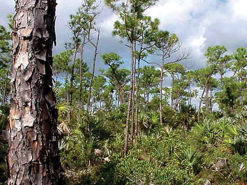
Figure 9. An example of developed areas in the Lower Florida Keys (Lopez Citation2001)
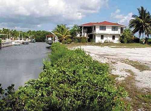
Figure 10. Flowchart of main processing steps used in the study
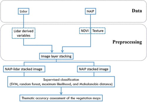
Figure 13. Individual input layers used to create both versions of the stacked image: the 2017 NAIP stacked image and the 2017 NAIP-2008 lidar stacked image (figures were modified from Mutlu et al. (Citation2008))
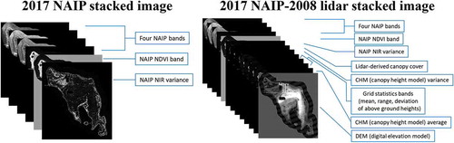
Figure 11. Flowchart explaining the steps used in the creation of the Canopy Height Model (CHM). a 3 m spatial resolution was used in ground estimation by considering the relatively low point density (approximately 2 points per m2) of the lidar data and the flat terrain of the study area
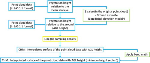
Figure 12. Examples of vertical profiles of lidar point clouds that depict different point structures in each area of (a) pinelands vegetation and (b) hammocks vegetation on No Name Key, Florida. The Quick Terrain Modeler® software was used in the creation of the vertical profiles
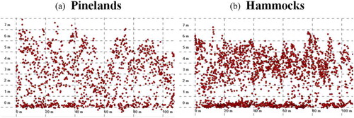
Table 1. Comparison of the statistics of the values in the original input bands and in the normalized bands in the 2 input images (2017 NAIP stacked and 2017 NAIP-2008 lidar stacked images). For the description of each band in each of the 2 input images, refer to
Table 2. The input layers used in the creation of the NAIP stacked image and the NAIP-lidar stacked image
Table 3. The 2 versions (original and normalized) for each of the 2 input image stacks (NAIP stacked and NAIP-lidar stacked) used in this study
Table 4. Depiction of the input using different classification output images in the accuracy assessment step. The accuracy of the total of 40 classified images was evaluated against the reference data collected on the 2017 NAIP-2008 lidar stacked image
Figure 14. The classified image of No Name Key, Florida with the best accuracy across the inputs and the classification algorithms. The 7 × 7 majority-filtered classification output from the Random Forest algorithm of the 2017 NAIP-2008 lidar stacked image with the original input bands (not with the normalized bands) achieved both the highest overall classification accuracy and the kappa coefficient (к)
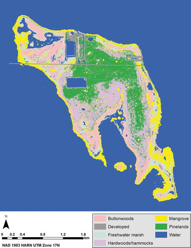
Figure 15. The classified image of No Name Key, Florida with the best accuracy for the 2017 NAIP stacked images. The best classification accuracy for the NAIP stacked image was achieved when using either the original or the normalized bands in the Support Vector Machine (SVM) classification with the new parameter values from García et al. (Citation2011) and applying a 7 × 7 majority filter. The above figure is the SVM classified image of the 7 × 7 majority-filtered 2017 NAIP stacked image with the original bands. It used the new parameter values from García et al. (Citation2011)
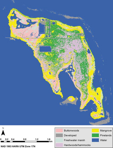
Figure 16. The classified images of No Name Key, Florida with the best and second best accuracies for the 2017 NAIP-2008 lidar stacked images. (a) The best classification accuracy for the NAIP-lidar stacked images was achieved when using the original bands in the Random Forest algorithm and applying a 7 × 7 majority filter. (b) The second best classification accuracy for the NAIP-lidar stacked images was achieved when using the original bands in the Support Vector Machine classification with the new parameter values from García et al. (Citation2011) and applying a 7 × 7 majority filter
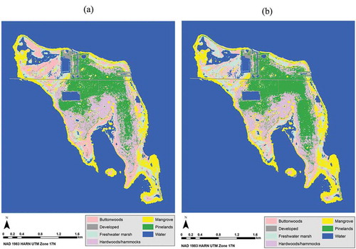
Figure 17. The plots that show the importance of each layer (or variable) in each of the 4 input images as estimated by the Random Forest algorithm. The variable importance of 100 indicates that the variable contributes the most in separating different land use/land cover classes from each other. Similarly, the variable importance of 0 indicates that the variable contributes the least. For the description of each band in each of the 4 input images, refer to either or
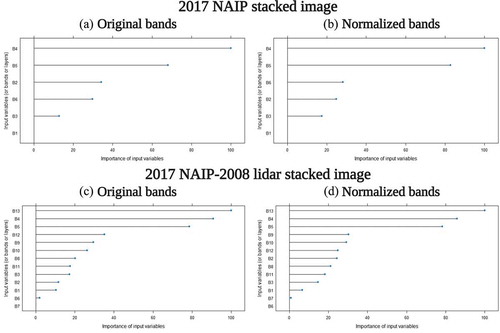
Table 5. Summary of the accuracy assessment results
Table 6. The confusion matrix generated by comparing the (7 × 7 majority filter-applied) Random Forest algorithm output on the 2017 NAIP-2008 lidar stacked image (with original bands) against the reference data
Table 7. The importance of each layera (or variable) in each of the 4 input images as estimated by the Random Forest algorithm, with 100 being the most important and 0 being the least important