Individual tree detection using template matching of multiple rasters derived from multispectral airborne laser scanning data

Figures & data

Figure 1. Study area and plot positions. Red polygon on the right is the laser-scanned area

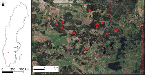
Table 1. Basic information about the 12 plots, including mean DBH and height, stem density, proportion of pine trees, and proportion of small trees. SD refers to standard deviation

Plot no.	Mean DBH (cm)	SD DBH/Mean DBH	Mean height (m)	SD height/Mean height	Number of stems/ha	Proportion of spruce/pine/deciduous (%)	Proportion of small trees (%)
1	30.2	0.24	21.8	0.16	615	93/1/6	24
2	28.3	0.24	21.2	0.17	704	95/0/5	27
3	24.4	0.24	19.7	0.17	921	68/3/29	28
4	22.6	0.33	18.3	0.25	905	85/0/15	29
5	28.8	0.29	21.2	0.2	740	91/0/9	31
6	27.4	0.22	19.5	0.15	635	49/49/2	32
7	28.2	0.29	20.9	0.21	543	93/0/7	35
8	28.3	0.36	20.7	0.25	820	92/0/8	38
9	21.5	0.38	17.6	0.28	899	77/1/22	44
10	22.2	0.35	17.9	0.25	808	49/0/51	46
11	17.1	0.42	14.7	0.33	1068	86/0/14	60
12	20.2	0.69	14.0	0.51	800	52/40/8	60

Figure 2. The DBH distribution of plots 1 − 12

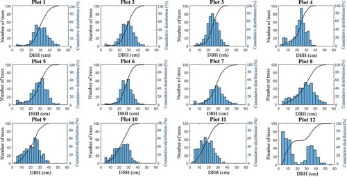
Figure 3. Corrections of the single-tree positions in a representative plot. (a) Measured tree positions. (b) Corrected tree positions. The background rasters represent the output of the smoothed nDSM. The black solid lines indicate the plot’s boundary. The dotted lines show the boundaries of the 20 m × 20 m subplots

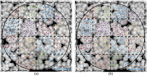
Figure 4. Framework of the ITD method tested here and questions considered when analysing the results

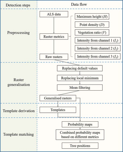
Figure 5. The flight and scanning direction of the MS-ALS data used in this study and the generated point cloud. (a) Flight and scanning direction (i) shown on a maximum height raster (ii). (b) The corresponding point cloud seen from different directions

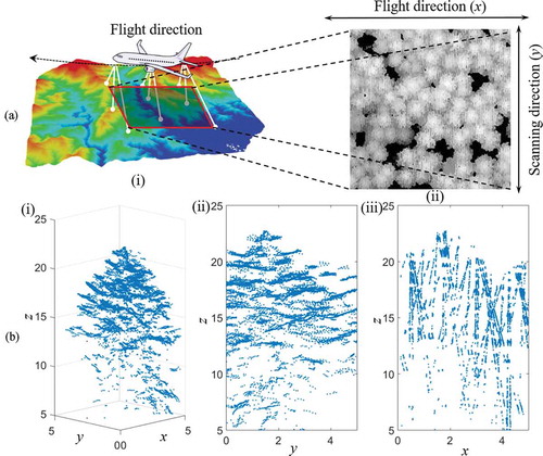
Figure 6. Templates (9 × 9) on a height raster image. (a) Initial positions of the nodes. (b) Final positions of the templates. Red boxes delineate the borders of the templates and blue spots indicate their centres. The background rasters are the M_DSM processed after the image generation steps proposed in.Section 3.2.1

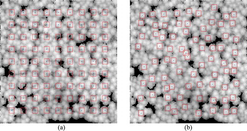
Figure 7. The similarity calculation process

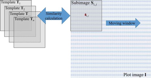
Figure 8. Similarly maps derived from different metrics by template matching. (a – e) H, D, V, I₁, I₂ and I_3. Red and blue indicate high and low values, respectively. Histogram equalization was performed to improve the visualization of the results

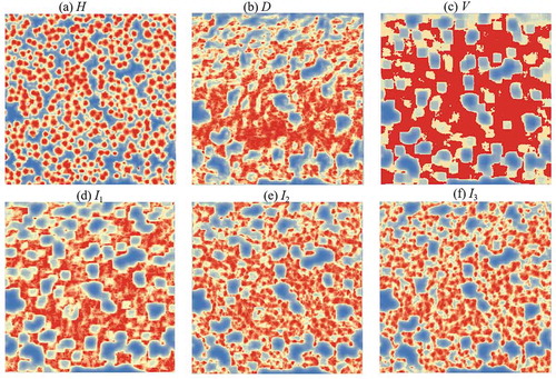
Figure 9. The effects of the processing steps on rasters based on different metrics within a 25 × 25 m area

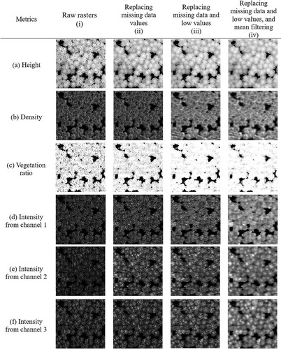
Figure 10. F-scores for all plots based on individual metrics: M_DSM, H, V, D, I₁, I₂ and I_3.

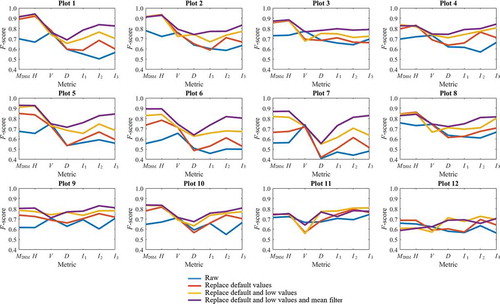
Figure 11. F-scores for detection using different numbers of templates

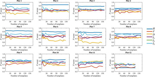
Figure 12. F-scores using different metrics/combined metrics for 12 plots

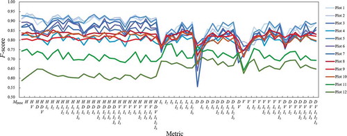
Figure 13. An example for a small tree standing beside a dominant tree in Plot 12. (a) 3D point cloud from laser data. (b) rasters of (i) H, (ii) D, (iii) I₂ and (iv) I₃. Red asterisks and blue circles indicate field-measured trees and detected trees, respectively; blue lines represent the links between them. Yellow cycle makes out the small tree in different rasters

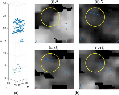
Figure 14. An example for several understorey trees standing under a dominant tree in Plot 12. (a) 3D point cloud from laser data. (b) rasters of (i) H, (ii) D, (iii) I₂ and (iv) I₃. Red asterisks and blue circles indicate field-measured trees and detected trees, respectively; blue lines represent the links between them

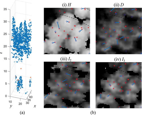
Figure 15. Similarity maps for (a) H, (b) I₂ and (c) D in Plot 12. Red and blue indicate high and low values, respectively; black points indicate the positions of trees according to field measurements

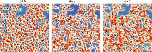
Figure 16. Linkage between trees detected by template matching and field-measured trees using the (a) H, (b) P_{I2, I3} and (c) P_{D, V} metrics for Plot 12. Red asterisks and blue circles indicate field-measured trees and detected trees, respectively; blue lines represent the links between them. The background rasters are the nDSM processed after the image generation steps proposed in.Section 3.2.1

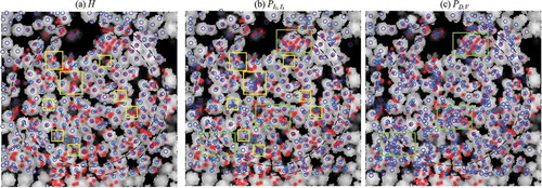
Table 2. Summary of the plot attributes, optimal metric combinations for single tree detection in each plot, the accuracy achieved using these combinations, and the accuracy achieved by direct detection based on local maxima for each plot

Plot no.	Proportion of small trees (%)	Template matching								Local maxima detection
		Option 1				Option 2
		Metrics	F-scores	RD	RD,s	Metrics	F-scores	RD	RD,s	F-scores	RD	RD,s
1	24	H	0.94	0.90	0.82	PH, I2, I3	0.93	0.90	0.82	0.91	0.87	0.72
2	27	H	0.93	0.89	0.68	PH, I2, I3	0.92	0.89	0.72	0.91	0.86	0.61
3	28	H	0.88	0.83	0.67	PH, I2, I3	0.88	0.86	0.73	0.87	0.81	0.64
4	29	H	0.83	0.73	0.42	PH, I2, I3	0.83	0.72	0.42	0.83	0.73	0.39
5	31	H	0.93	0.89	0.69	PH, I2, I3	0.93	0.89	0.75	0.93	0.89	0.72
6	32	PH, I2, I3	0.90	0.88	0.83	PH, I2, I3	0.90	0.88	0.83	0.89	0.87	0.84
7	35	PH, I2, I3	0.91	0.89	0.77	PH, I2, I3	0.91	0.89	0.77	0.87	0.90	0.75
8	38	PV, I2, I3	0.85	0.79	0.60	PH, I2, I3	0.84	0.75	0.52	0.83	0.72	0.47
9	44	PV, I2, I3	0.85	0.77	0.65	PI2, I3	0.85	0.81	0.72	0.80	0.73	0.52
10	46	PV, I2, I3	0.85	0.84	0.74	PI2, I3	0.84	0.87	0.81	0.84	0.73	0.56
11	60	I3	0.78	0.69	0.59	I2	0.77	0.70	0.61	0.74	0.61	0.46
12	60	PD, V	0.73	0.68	0.56	I2	0.69	0.59	0.46	0.59	0.44	0.24