Figures & data
Figure 1. Vector triangles illustrating cluster method for resolving the heading direction ambiguity and estimating airspeed and wind. In this example, the wind speed is twice the insect’s airspeed. (a) Vector triangles for two insects with different headings. (b) Resolution of ambiguity from available measurements for two insects with no random variation. (c) Resolution for multiple insects with random variation; for clarity, only the endpoints (green dots) of the track vectors are shown. Diagonal crosses indicate the centroids of the two sets of blue points. Key: N, north; O, origin (where speeds are zero); A, alignment of insect; F, flight of insect through the air; T, track of insect; W, wind; m, a measured value, e, an estimated value
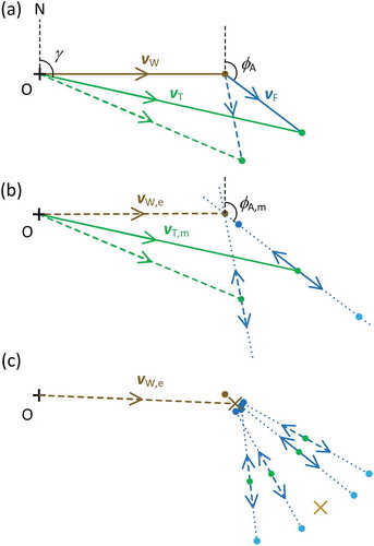
Figure 2. Vector triangles illustrating the projection method for resolving the heading direction ambiguity and estimating airspeed and wind. Scenario and symbols as in . (a) As (a), with alternative flight and track vectors shown in paler colours. (b) Projections of the flight vectors onto the mean alignment direction φA,av and the normal to this direction. (c), (d) Projections of both the flight vectors and the track vectors onto the normal for, respectively, the original (φA,m,i) and the alternative (φA,m,i + 180°) sets of heading directions. For clarity, most track vectors are omitted, but all track-vector endpoints are indicated with green dots; the m subscript (indicating measurement) has also been dropped
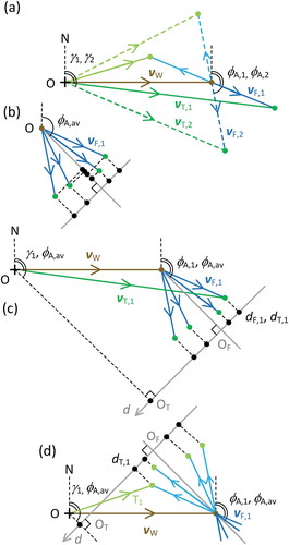
Figure 3. Cluster- and projection-method analyses of large-moth echoes observed at heights of 475 to 625 m between 01.00 and 02.00 h on 14 September 2007. (a) Distribution of track speeds; (b) distribution of track directions; (c) distribution of alignments; (d) formation of along-track (A, dark blue) and back-track (B, light blue) alignment groups and elimination of outliers (grey, also indicated in (a) and (b)); mean directions and the range ±1 SD are shown inside the circle in (b) and (d); (e) track velocity endpoints (green) relative to origin O (larger cross, where insect velocity is zero), and centroid of endpoints (smaller cross); (f) putative-wind velocity endpoints for A and B groups, and centroids (with centroid of selected group circled in red); (g) variation of A and B group RMSs with assumed airspeed, with selected airspeed/group combination circled in red; (h) scatterplot of flight- and track-vector projections onto normal to the mean heading direction, and linear regression fit
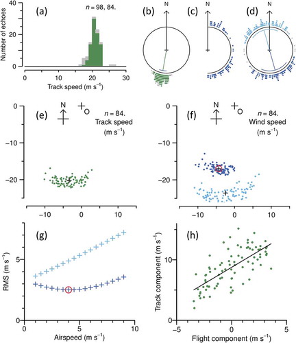
Figure 4. Track directions (green) and alignments (blue) and their SDs, and resolved headings (dots), for large moths at Bourke, NSW, during the night of 13–14 September 2007. Track direction mean and SD represented as in (b); length is arbitrary. Alignment represented by hourglass symbol, width of which indicates the ±1-SD range of the alignment distribution. Large dots indicate heading resolved by projection method, blue if p ≤ 0.05 and grey if 0.05 < p ≤ 0.2; small black dots indicate heading closest to track direction. Numbers are sample size for the unit. Key: Du, dusk (end of civil twilight, 18.31 h); Da,dawn (05.53 h). Note: observations ceased at 05.00 h
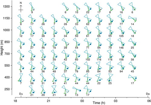
Table 1. Performance of different heading-resolution methods
Figure 5. Wind speeds and directions inferred from projection-method analyses of large-moth echoes (orange, paler for units with 0.05 < p ≤ 0.2) and from dynamic downscaling of meteorological observations via TAPM (violet), for the night of 13–14 September 2007 at Bourke, NSW. Boxes at end of large-moth inferred-wind arrows indicate ±1-SD ranges of individual wind speed and direction estimates. Number of echoes in each unit as in
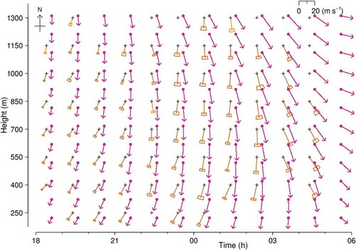
Figure 6. Features of the analysis results for 15 nights of intense large-moth migration at Bourke, NSW, in September and October 2007, for units with the heading resolved at p ≤ 0.2. (a), (b) Relation of the SD of the inferred wind direction to the SD of the measured track (a) and heading (b) directions, n = 716 (after elimination of 8 units with outlier SDs); solid lines indicate regression fits. (c) Relation of p-values (logarithmically transformed) of the cluster (pF) and projection (pb) methods, n = 498 (with units with both p-values < 0.0001 excluded); solid line indicates equal p-values, dashed lines indicate p = 0.05 (left) and p = 0.2 (right). (d) Histogram of crab angle χ, n = 724
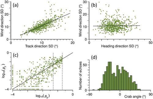
Figure 7. Relation of wind estimated from radar observations of insects to wind from meteorological observations downscaled via TAPM. Data from 15 nights as in Figure 6, n = 724 for speeds (a) and 718 for directions (b). Dashed line indicates where the two quantities are equal, solid line is regression fit (linear in (a), circular-circular in (b))
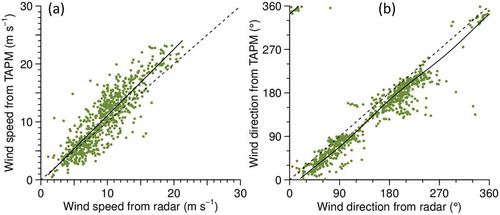
Figure 8. Resolution of heading direction by assume-along and subtraction methods, for same dataset as that of Figures 4 and 5 (and using same symbols). Key: blue, alignment and its SD; green, track vector and its SD; violet, TAPM wind vector (interpolated to mean height for unit); red or black without arrowhead, flight vector (heading and airspeed) inferred by vector subtraction; black dot,heading resolved by assume-along method; yellow fill,heading resolved by subtraction method. For visibility, flight vectors with speeds < 3 ms–1 are shown as 3 ms–1 and coloured black instead of red
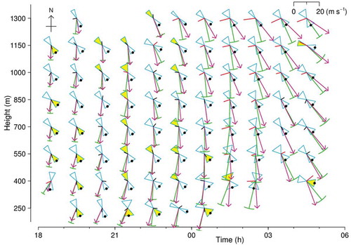
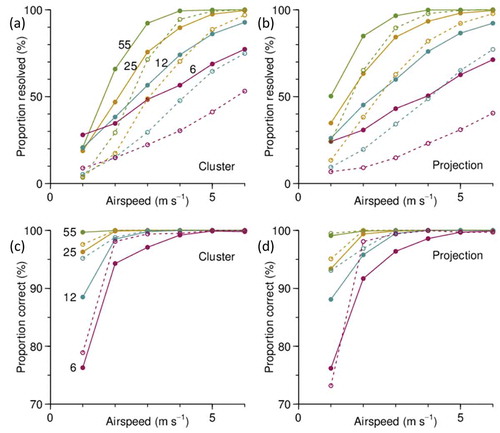
Figure 9. Simulation results for unit at 02 h (start time) and 1000 m on 14 September 2007 and an airspeed of 4 ms–1, showing variations with heading angle and sample size. E indicates the 90° direction (towards E) of the simulated wind. Samples sizes ns were 55 (as in actual unit, after removal of outliers), 25, 12 and 6. (a) Mean (point) and standard error on the mean (bars) over 100 replicates for F-test p-value from cluster-method analyses. Dashed lines indicate p = 0.2 and p = 0.05. (b) Proportion of the 100 replicates resolved by the cluster method at p ≤ 0.2. Short dashed lines indicate average over the 12 heading directions for the proportion resolved at p ≤ 0.05. (c), (d) Same as (a), (b) for projection method; p-value is now that for the regression slope parameter b.
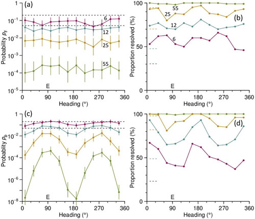
Figure 10. Simulation results for airspeeds in the range 1 to 6 ms–1, for same unit and sample sizes as in Figure 9. (a), (b) Proportion of units resolved by cluster method and projection method. (c), (d) Proportion of units resolved by these two methods for which the assignment is correct. Results at p ≤ 0.2 indicated by solid lines, at p ≤ 0.05 by dashed lines