Figures & data
Figure 1. Holistically nested edge detection (HED) architecture. Three spectral bands from every satellite image are selected as HED input. Input images are fed through five distinct stages of image convolution, and between each stage, a max pooling layer decreases image size. The squares to the bottom left of the image detail the number of convolution kernels at each stage. The side outputs are resized and optimally fused to generate the output.
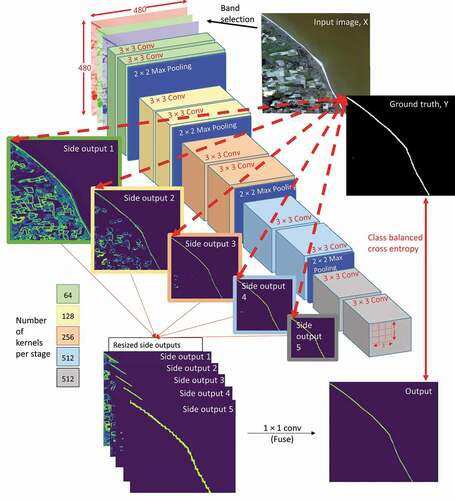
Figure 2. Overview of the three stages carried out in this study. Four holistically nested edge detection (HED) models were independently trained using different spectral band combinations (training). The performance of each HED model was evaluated using a separate image set (validation). The best performing HED model, trained on images with spectral band combination red, green, near-infrared (RG-NIR), formed the VEdge_Detector tool. This tool detected the vegetation line position from multiple images of the same shoreline captured over a 10-year period (shoreline change detection).
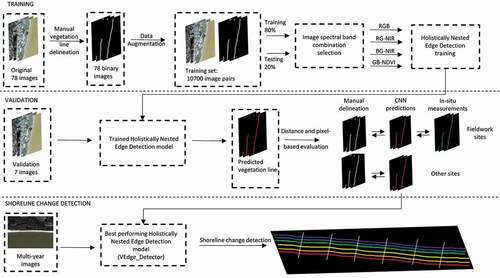
Figure 3. Transformations used in data augmentation (a) original image (cropped to 480 × 480 pixel size), (b) – (d) original image rotated by 90°, 180°, and 270°, (e) original image flipped vertically, (f)–(h) flipped image rotated by 90°, 180°, and 270°, (i)–(l) Gaussian noise added to the flipped images. Transformations (b)–(h) were simultaneously conducted on the binary images.
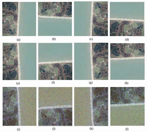
Figure 4. Example of 0.05 (yellow), 0.55 (orange), and 0.95 (red) confidence contours produced by VEdge_Detector at Winterton, UK. The confidence contours were generated from the raw VEdge_Detector output, which is overlaid as the blue colour ramp. Light and dark blue pixels represent the locations predicted as being an edge pixel with a high and low confidence, respectively. The manually digitized vegetation line (black) is displayed for visual comparison. Land and sea are found to the left and right of the image, respectively. Aerial imagery, provided by the Environment Agency with 40 cm resolution, is used as a backdrop (Environment Agency, Citation2020).
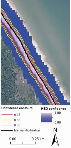
Table 1. Locations of holistically nested edge detection validation images. Other columns provide information on dominant shoreline direction, spring and neap tidal ranges, dominant sediment type, geomorphology, and climate at each site as well as whether ground-referenced measurements of the coastal vegetation edge were collected
Figure 5. (a) Original 3 m PlanetScope image of Cromer, Norfolk, UK (52°93ʹ58.3 N, 1°27ʹ18.0 E). Predicted coastal vegetation edge locations using the HED model trained with spectral band combination (b) RGB, (c) RG-NDVI, (d) RB-NIR, (e) RG-NIR.
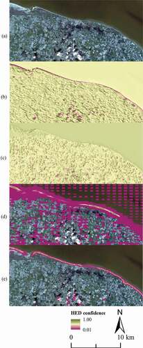
Figure 6. (a) Original 5 m RapidEye image of Varela, Guinea-Bissau (12°28ʹ61.0 N, −16°59ʹ45.7 E). Predicted coastal vegetation edge locations using the HED model trained with spectral band combination (b) RGB, (c) RG-NDVI, (d) RB-NIR, (e) RG-NIR.
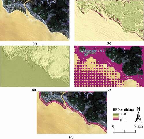
Figure 7. (a) Original 3 m PlanetScope image of the islands of Sylt, Amrum, and Föhr, Frisian Islands, Germany (54°68ʹ31.4 N, 8°55ʹ74.4 E). Predicted coastal vegetation edge locations using the HED model trained with spectral band combination (b) RGB, (c) RG-NDVI, (d) RB-NIR, (e) RG-NIR.
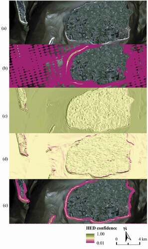
Table 2. VEdge_Detector accuracy at the three field sites determined by pixel and distance-based metrics from ground-referenced measurements. Shaded pixels in the mean absolute error column represent a landward (green) or seaward (blue) bias respectively in VEdge_Detector predictions. Darker colours represent a greater landward or seaward bias. Red boxes indicate the confidence contours with lowest RMSE and MAE per site. VEdge_Detector outputs are shown in
Figure 8. Comparison of VEdge_Detector tool predictions to field measurements of vegetation line at (a) Covehithe, (b) Walberswick, and (c) Dunwich. Locations of photograph (a)i, (b)i, and (c)i are show by arrows on corresponding images. The solid black lines show the ground-referenced vegetation lines at all sites. At Walberswick, the landward and seaward vegetation lines derived from field measurements are denoted by a solid and dashed line, respectively.
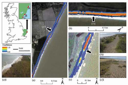
Table 3. VEdge_Detector accuracy at the four validation sites without ground-referenced data determined by pixel and distance-based metrics. Shaded pixels in the mean absolute error column represents a landward (green) or seaward (blue) bias respectively in VEdge_Detector predictions. Darker colours represent a greater landward or seaward bias. Red boxes indicate the confidence contours with lowest RMSE and MAE per site. VEdge_Detector outputs are shown in
Figure 9. VEdge_Detector outputs for (a) Winterton, Suffolk, UK (b) A stretch of Bribie Island, Australia, separate to the locations used for training outlined in the supplemental material, and (c) Perranuthnoe, Cornwall, UK. The red oval indicates the rocky cliff section where the VEdge_Detector failed to detect cliff top vegetation, (d) Wilk-Ann-zee, Netherlands. (a) and (b) display the predicted vegetation line in red with a confidence ≥0.95. (c) and (d) show examples of all VEdge_Detector outputs prior to applying any confidence thresholding. The white line in (c) and (d) shows the location of the manually digitized line.
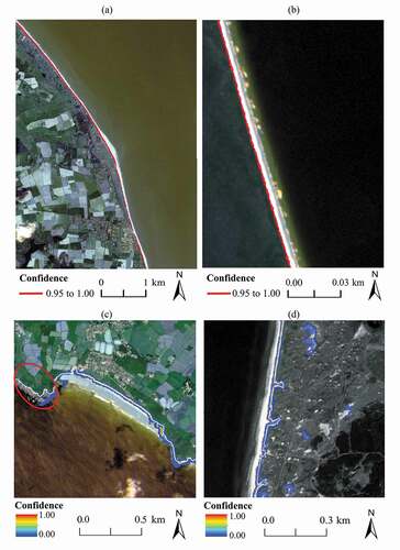
Figure 10. (a) VEdge_Detector outputs for a 2010 (red) and 2020 (purple) image of the Covehithe cliffs, Suffolk. Darker colours represent pixels predicted as the vegetation line with a higher confidence. Inset graphs, comparison of vegetation curves at transects situated at location i (smallest recorded change in shoreline position) and ii (largest recorded retreat in shoreline). Note: The image shows VEdge_Detector outputs with confidence values from 0.01 to 1.00, whereas the graphs show values 0.05–1.00 because the line graphs substantially ‘fan’ between 0.01 and 0.05. (b) Rates of landward retreat (End Point Rate) at Covehithe between 2010 and 2020.
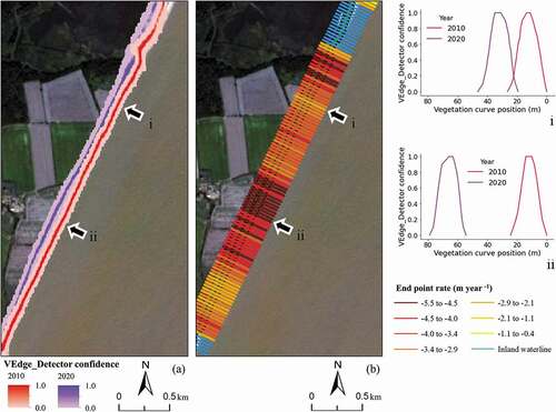
Figure 11. Top: Vegetation confidence curve position during years 2010–2020 at one transect. Bottom: Representation of vegetation curves as a line. Dots represent locations of the 0.95 confidence contours, vertical lines represent locations of the 0.05 confidence contours. Insets i and ii: Transect location and all pixels predicted as the vegetation line with confidence >0.95 overlaid on the 2020 image. Pixel colour coding by year is consistent with line graphs. Some of the colours are occluded in the image due to overlap.
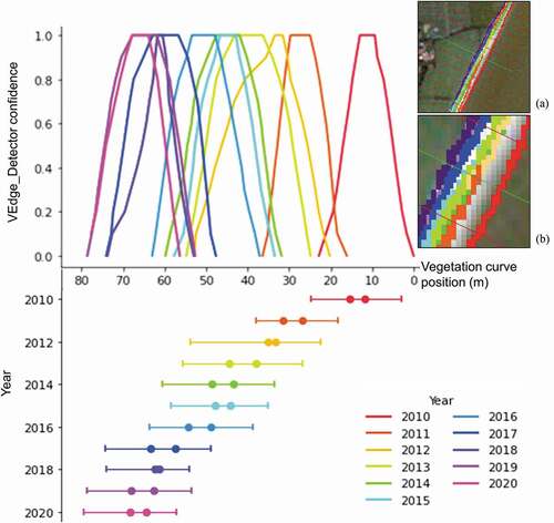
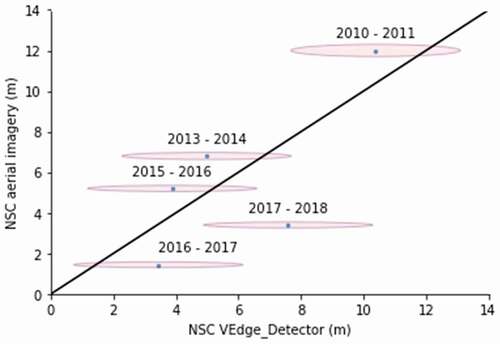
Figure 12. Comparison of Net Shoreline Change (NSC) values generated the VEdge_Detector 0.95 confidence contours and manually digitized aerial imagery. The blue dots show annual NSC values for the whole of the Covehithe coastline averaged over all orthogonal transects. The ovals represent the error associated with the two methods. The black line shows the position of the blue dots if there was an exact match between NSC values generated using the two methods.