Figures & data
Figure 1. Location of the study area and the sample fields included in the work for which yield measurements were conducted. Note that five fields were monitored in both 2018 and 2019. The zoom at the top left highlights the presence of trees in the fields. Bing Maps images are displayed in the background
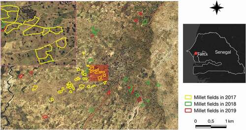
Figure 2. Per year distribution of the millet yields over sample fields showing a high year-to-year variability. Overall, recorded yield values in 2018 are lower than in 2017 and 2019 and most of these values are distributed around 900 kg/ha, contrary to other years where the values are more uniformly distributed
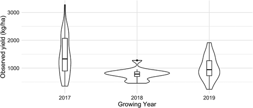
Figure 3. Overview of the acquisition dates of Sentinel-1 (S1) and Sentinel-2 (S2) images over three agricultural seasons. S2 acquisitions are sparsed due to the ubiquitous cloudiness
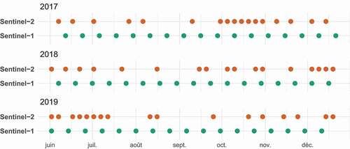
Table 1. Vegetation indices derived from optical bands (Band abbreviations: B–Blue, G–Green, R–Red, RE–Red edge, NIR–Near Infrared, SWIR–Short Wavelength Infrared)
Figure 4. Candidate and final patches for the spatialization of millet yields over 2018 and 2019 growing seasons. Bing Maps images are displayed in the background of subfigures 4e and 4f. The maps were created with https://www.qgis.org/fr/site/forusers/download.htmlQGIS 3.14
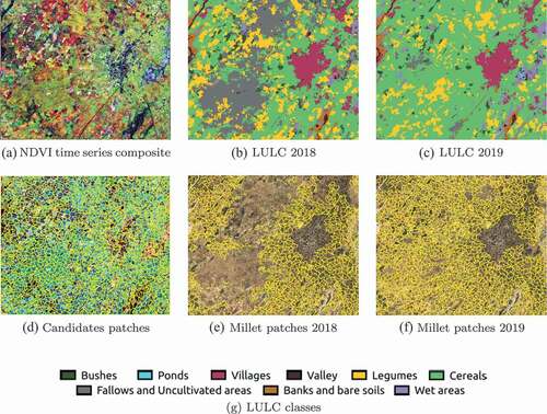
Table 2. Characteristics of the ground truth data used for LULC mapping
Table 3. Hyperparameter settings of the different approaches considered for millet yield estimation. RR and RF hyperparameters were optimized by varying associated values while MLP, LSTM, and CNN hyperparameters were empirically fixed
Table 4. Details of the CNN architecture: Conv stands for Convolution operation, is the number of filters,
is the kernel size,
is the stride value, and
is the activation function. As for precedent neural network models, we used a maximum number of filters of 64
Figure 5. Scatter plots of the observed versus predicted millet yields averaged over the 10 repeated 3-fold cross validation procedure considering Ridge Regression (RR), Random Forest (RF), Multi-Layer Perceptron (MLP), Long Short-Term Memory (LSTM), and Convolutional Neural Network (CNN) models and the set of predictor variables (i.e. SAR, optical, and VI)
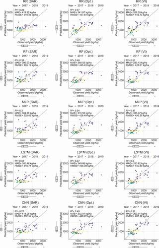
Table 5. Average performances of the Linear Regression (LR), Ridge Regression (RR), Random Forest (RF), Multi-Layer Perceptron (MLP), Long Short-Term Memory (LSTM) and Convolutional Neural Network (CNN) models over the 10 repeated 3-fold cross validation procedure. The baseline (LR model) was performed using the maximum observed NDVI value over the growing cycle as unique predictor
Figure 6. Average performances (standard deviation as error bar) of Ridge Regression (RR), Random Forest (RF), Multi-Layer Perceptron (MLP), Long Short-Term Memory (LSTM), and Convolutional Neural Network (CNN) models over the 10 repeated 3-fold cross validation procedure considering the four combination scenarios of predictor variables (i.e. SAR+Optical, SAR+VI, Optical+VI, SAR+Optical+VI). We referred to as ‘Best mono-source’ the best performances obtained from individual feature set (within optical and VI time series)
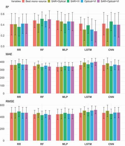
Figure 7. Average performances (considering and Relative RMSE metrics) of the Random Forest (RF) model with SAR and VI combination as input for forecasting millet yields from the emergence to senescence stage via time windows shortened by 15-day increments from the beginning. The x (resp. y) axis represents the beginning (resp. the end) of the time window
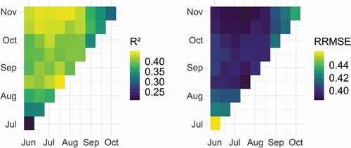
Figure 8. Millet yield mapping and gap between forecasts and estimates for 2018 and 2019 agricultural seasons using the Random Forest (RF) model and SAR as well as VI combination as input. Yield forecasting was achieved at mid October. A quantile discretization was applied to the maps. Bing Maps images are displayed in background. The maps were created with https://www.qgis.org/fr/site/forusers/download.htmlQGIS 3.14
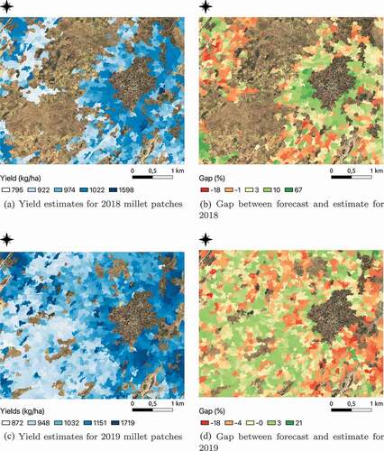
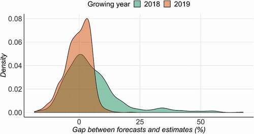
Figure 9. Distribution of gaps between yield forecasts and yield estimates for 2018 and 2019 millet patches. Most of the prediction errors are low