Assessing spatial variability and estimating mean crown diameter in boreal forests using variograms and amplitude spectra of very-high-resolution remote sensing data

Figures & data

Figure 1. Map of Finland and its boreal forest vegetation zones. Our study site is located in the vicinity of Hyytiälä forestry field station (61°50'44”N, 24°17'10”E) in the southern boreal forest zone.

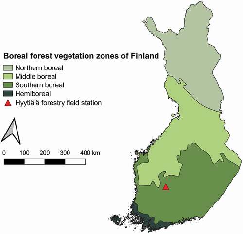
Table 1. Forest data for the test areas. The main tree species is indicated by the name of the test area. The coordinates in the centre point column correspond approximately to the centre of each test area

Test area	Centre	Basal	Stem	Mean	Crown
	point	area	count	height	diameter
	(lat, long)	(m^2 ha^–1)	(stems ha^–1)	(m)	(m)
pine 1	61°50'30”N, 24°18'29”E	19.8	921	17.1	3.4
pine 2	61°50'09”N, 24°20'50”E	23.4	643	21.0	4.0
pine 3	61°48'21”N, 24°20'29”E	20.7	556	20.5	4.1
pine 4	61°51'41”N, 24°16'14”E	21.9	795	18.3	3.3
pine 5	61°51'41”N, 24°15'22”E	18.1	1336	13.2	2.9
pine 6	61°51'25”N, 24°14'40”E	25.7	875	20.7	3.7
pine 7	61°49'24”N, 24°20'06”E	15.1	626	16.8	3.4
pine 8	61°49'29”N, 24°19'56”E	29.6	679	23.6	4.2
pine 9	61°51'37”N, 24°15'44”E	20.2	1449	13.6	2.8
spruce 1	61°49'28”N, 24°18'39”E	36.2	636	27.0	4.9
spruce 2	61°50'31”N, 24°16'16”E	22.5	1010	17.6	3.5
spruce 3	61°50'43”N, 24°18'01”E	34.8	632	26.1	4.9
spruce 4	61°49'34”N, 24°21'51”E	33.9	711	24.7	4.5
spruce 5	61°51'05”N, 24°17'01”E	32.3	616	26.2	4.8
spruce 6	61°49'35”N, 24°18'50”E	37.4	639	27.2	5.0
spruce 7	61°49'46”N, 24°20'31”E	33.8	896	22.6	4.0
spruce 8	61°50'26”N, 24°20'03”E	31.7	698	24.3	4.5
spruce 9	61°49'21”N, 24°22'00”E	32.0	669	24.2	4.3
larch	61°51'01”N, 24°18'04”E	19.4	669	20.7	5.6
broadleaved	61°50'36”N, 24°18'53”E	16.9	1070	18.2	4.5

Figure 2. The hyperspectral AISA image was used to determine suitable forest areas for our test areas, which had a size of $70\mathrm{m}\times 70\mathrm{m}$.

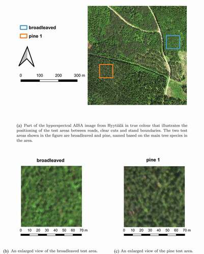
Table 2. The values of the canopy spectral variables for the two scenarios used in the Monte Carlo simulations. The used wavelength was 835 nm

	Understorey reflectance	Leaf reflectance	Leaf transmittance	Direct-to-global irradiance ratio
ideal	0.0	0.476	0.426	1.0
realistic	0.283	0.476	0.426	0.883

Figure 3. Flowchart of the used methodology. The same methods were also used for the simulated images.

Figure 4. Variogram analysis for test area ‘pine 8’ ($\lambda =835$ nm).

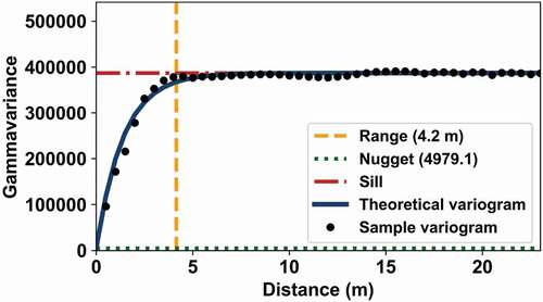
Figure 5. Relationships between the allometric mean crown diameters of the test areas and the estimations from (a) variogram and (b) amplitude spectrum analyses. The metrics used in the graphs are Pearson correlation coefficient (r), root-mean-square error (RMSE), and relative root-mean-square error (rRMSE).

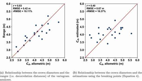
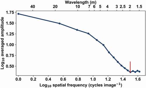
Figure 6. Averaged amplitude spectrum of measured reflectance (λ = 835 nm) for the test area ‘spruce 6’ in log-log coordinates. The red line corresponds to the visually located breaking point at 2.35 m.

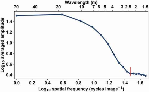
Table 3. Connection between the absolute estimation errors of the variogram analyses and the forest characteristics of our test areas (Table 1)

Forest variable	Basal area (m^2 ha^−1)	Stem count (stems ha^−1)	Mean height (m)	Crown diameter (m)
Pearson correlation coefficient (r)	-0.10	-0.15	0.13	0.50

Figure 7. Monte Carlo simulated forest of Plot 1 (‘realistic’ scenario). The simulated forest can be seen at the centre of the image with spatial dimensions of 70 m $\times$ 70 m. Measured reflectance data by the hyperspectral AISA imager was used as visualisation on the background. The used wavelength for the spectral data was 835 nm. Note that we used birch leaf spectrum for all modelled trees, whilst most of the real trees in the AISA image are conifers with lower 835 nm reflectance. We also traced $2\times {10}^9$ photons to ensure low Monte Carlo noise in the images.

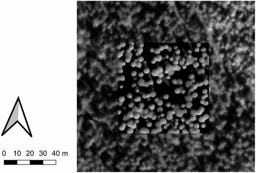
Table 4. Ranges of the variograms of the simulated forest images. ‘Ideal’ and ‘realistic’ describe the used simulation scenarios (Table 2)

Plot name	Crown	Range,	Range,
	diameter (m)	ideal (m)	realistic (m)
Plot 1	4.6	4.5	4.9
Plot 2	3.7	5.7	5.6
Plot 3	4.1	4.3	4.4
Plot 4	5.2	5.2	4.6
Plot 5	3.5	3.2	3.4
Plot 6	4.8	5.4	5.3
Plot 7	5.4	5.6	5.5

Figure 8. Averaged amplitude spectrum of simulated reflectance for ideal ‘Plot 4’. The spectrum does not show any clear structure in the high frequencies. The estimation accuracy for the mean crown diameter using variogram was 0.0 m for the same simulated image (Table 4).

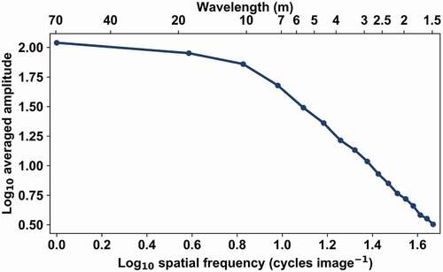
Figure A1. One of the additional test regions, which were used to test the hypothesis. Mean crown diameter for the forested area was 3.6 m.

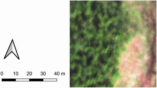
Figure A2. Variogram analysis for one of the additional test regions ($\lambda =835$ nm). The analysis did not succeed for the partly logged forest area.

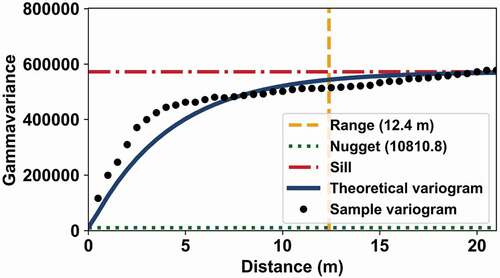
Figure A3. Averaged amplitude spectrum of measured reflectance ($\lambda =835$ nm) for one of the additional test regions in log-log coordinates. The red line corresponds to the visually located breaking point at 1.98 m.