Early validation study of the photochemical reflectance index (PRI) and the normalized difference vegetation index (NDVI) derived from the GCOM-C satellite in Mongolian grasslands

Figures & data

Figure 1. The national-scale target area and the locations of the ground sites (red triangles). The backdrop image is a GCOM-C/SGLI false colour image, with the water bodies painted in sky blue.

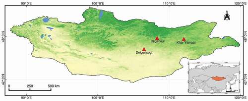
Figure 2. Satellite and on-site camera images of the ground sites: (a) Baganuur: BGN, (b) Delgertsogt: DGT, and (c) Khar yamaat: KYM. Satellite images were created from Sentinel-2A true colour images with the red squares representing the 500 m × 500 m areas covering the sites.

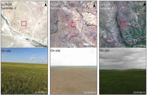
Table 1. Descriptions of the ground sites and the dates of in-situ and satellite observations.

Site ID	Site name	Latitude^1, longitude^1, altitude	Dominant vegetation species	Observation date^2 and local time
				in-situ	Satellite (SGLI)	Satellite (MODIS)
BGN	Baganuur	47°47‘53.3’’ N, 108°19‘51.5’’ E, 1396 m	Agropyron cristatum, Artemisia spp., Chenopodium spp., Cleistogenes squarrosa, Stipa krylovii	2018-08-22,　16:37–16:38 2018-08-23,　08:37–18:03 2018-08-24,　07:35–12:33	2018-08-24, 11:39	2018-08-24, 13:39
DGT	Delgertsogt	46°14‘56.0’’ N, 106°29‘42.9’’ E, 1380 m	Allium spp., Artemisia spp., Carex spp., Chenopodium spp., Salsora spp., Stipa krylovii	2019-08-08,　13:20–14:46 2019-08-09,　10:44–12:16	2019-08-09, 11:54 2019-08-10, 11:27	2019-08-09, 12:04 2019-08-10, 11:44
KYM	Khar yamaat	47°40‘13.8’’ N, 112°4‘34.9’’ E, 1060 m	Allium spp., Artemisia spp., Chenopodium spp., Cleistogenes squarrosa, Elymus chinensis, Potentilla acaulis, Stipa spp.	2019-08-13,　07:15–09:24	2019-08-13, 11:47	2019-08-13, 12:03

^aLatitude and longitude depict the location of the centres of the sites, described in WGS84.

^bDate is written according to ISO 8601.

Figure 3. Transect lines and satellite pixels (Table 4) corresponding to the in-situ spectral observation points at the (a) BGN, (b) DGT, and (c) KYM sites. Black dots denote the spectral observation points. Black lines denote the transect lines. Blue and orange squares denote the 250 m × 250 m area around the pixel centres of the SGLI and MODIS images, respectively. (d) a picture of an in-situ spectral observation.

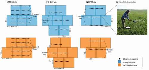
Table 2. Satellite data used in this study.

Satellite/sensor	Products	Spatial resolution	Version and period
GCOM-C/SGLI	GC1SG1 product Level 2 − Daily: NDVI; band reflectance of VN05^1, VN06, VN08, VN11, − 8-day statistics: NDVI (max); VN08 (max); VN11 (max)	250 m	Version 1 (1001): Jan. 2018–June 2019, Version 2 (2000): July 2019–Dec. 2019
Terra/MODIS	MOD09GQ − Daily: sur_refl_b01; sur_refl_b02,	250 m	Collection 6: 2018 and 2019
	MOD09Q 1− 8-day composite: sur_refl_b01; sur_refl_b02,
	MOD13Q1 − 16-day composite: NDVI
	MODOCGA − Daily: sur_refl_b11; sur_refl_b12	1000 m	Version 6: 2018 and 2019

^a‘VN’ is a prefix for GCOM-C SGLI band name, meaning ‘visible and near infrared’.

Figure 4. Relative spectral response (RSR) of SGLI (blue) and MODIS (yellow) in the wavelength between 500 nm 900 nm, along with typical examples of spectral reflectance of ground covers: grass canopy, dry grass canopy, dry soil, and wet soil. The reflectances of grass (LAI = 1.05) and dry grass (LAI = 0.18) canopies were measured at the Khar yamaat and Baganuur sites, respectively (in this study). The “dry grass canopy” means that the ground was covered with dry soil and sparse grass. The reflectance of the forest canopy was measured at a deciduous broad-leaved forest in Takayama, Japan (obtained from the Phenological Eyes Network, Nasahara and Nagai, 2015). The reflectance data from dry soil and wet soil was obtained from the literature (Baumgardner et al., 1986).

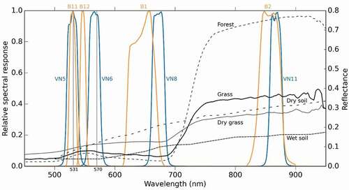
Table 3. The satellite products used for deriving the satellite vegetation index (VI) and band reflectance (BR).

VI and BR	Sensor	Temporal resolution	Methods to obtain the VI and BR	Corresponding figures
PRI	SGLI	daily	calculated from band reflectance (VN5; VN6)	Figs. 7, 9, 11, 12
	MODIS	daily	calculated from band reflectance (band 11 and 12 of MODOCGA)	Figs. 7, 11
NDVI	SGLI	daily	calculated from band reflectance (VN8; VN11)	Figs. 6, 12
		8-day	8-day maximum of daily NDVI (mentioned above)	Figs. 7, 13
		annual	annual maximum of JAXA 8-day NDVI product	Figs. 14, 15
	MODIS	daily	calculated from band reflectance (band 1 and band 2 of MOD09GQ)	Fig. 6
		8-day	8-day maximum of daily NDVI (mentioned above)	Figs. 7, 13
		annual	annual maximum of NASA 16-day NDVI product (MOD13Q1)	Figs. 14, 15
BR	SGLI	daily	JAXA daily product (VN5; VN6; VN8; VN11)	Fig. 12
		8-day	JAXA 8-day product (max VN8; max VN11)	Fig. 7
	MODIS	daily	MODOCGA (band 11; band 12)	Fig. 7
		8-day	MOD09Q1 (band 1; band 2)	Fig. 7

Table 4. Coordinate of the pixels within the satellite product tile (04, 25) (vertical tile number, horizontal tile number) used in this study.

Site	Sensor	Sample size	Row and column within the 0425 tile
BGN	SGLI	5	(1056, 1329), (1056, 1330), (1057, 1330), (1057, 1331), (1057, 1332)
	MODIS	6	(1056, 1328), (1056, 1329), (1056, 1330), (1057, 1329), (1057, 1330), (1057, 1331)
DGT	SGLI	7	(1799, 1747), (1799, 1748), (1800, 1748), (1800, 1749), (1800, 1750), (1801, 1751), (1801, 1750)
	MODIS	7	(1799, 1747), (1799, 1748), (1800, 1748), (1800, 1749), (1800, 1750), (1801, 1750), (1801, 1751)
KYM	SGLI	5	(1117, 2624), (1117, 2625), (1118, 2625), (1118, 2626), (1118, 2627)
	MODIS	5	(1117, 2624), (1117, 2625), (1117, 2626), (1118, 2626), (1118, 2627)

Figure 5. Workflow to acquire the in-situ vegetation index (VI, PRI, and NDVI).

Figure 6. Comparison of the in-situ NDVI and the satellite NDVI: (a) GCOM-C/SGLI and (b) Terra/MODIS. The satellite NDVI was taken on the closest sunny day to the day of the in-situ observation. The RMSE for all data was calculated using 1) BGN, DGT (satellite data on 2019-08-09), and KYM data and 2) BGN, DGT (satellite data on 2019-08-10), and KYM data. For the DGT site, the satellite NDVI of two days (the closest sunny day for both SGLI and MODIS: 2019-08-10 and the same day with the in-situ observation: 2019-08-09, cloudy for SGLI and sunny for MODIS) was demonstrated. The bar denotes the uncertainty of the in-situ mean PRI calculated by Eq. 6(6) $\sigma =\frac{2y}{{\left(x+y\right)}^2}\sqrt{{{\sigma }_x}^2+{{\sigma }_y}^2.}$(6) .

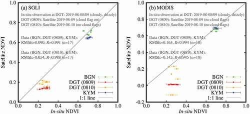
Table 5. The correlation coefficient and the root-mean-square error between the in-situ vegetation index (VI) and satellite VI at each observation site.

Site	In-situ observation	Satellite		NDVI		PRI
	Date, condition	Sensor	Date, condition	RMSE	R	RMSE	R
BGN	2018-08-22/24, sunny	SGLI	2018-08-24, no cloud	0.033	0.048	0.052	−0.76
		MODIS	2018-08-24, no cloud	0.027	0.53	NA	NA
DGT	2019-08-08/09, cloudy, drizzly	SGLI	2019-08-09, cloud	0.128	0.66	0.021	−0.48
			2019-08-10, no cloud	0.078	−0.017	0.047	0.42
		MODIS	2019-08-09, no cloud	0.259	−0.20	NA	NA
			2019-08-10, no cloud	0.231	−0.21	NA	NA
KYM	2019-08-13, sunny	SGLI	2019-08-13, no cloud	0.062	0.96	0.069	0.52
		MODIS	2019-08-13, no cloud	0.016	−0.89	NA	NA

Table 6. Comparison of NDVI_SGLI and NDVI_MODIS simulated using the spectral reflectance of a forest canopy, grass, dry grass, wet soil, and dry soil, which is described in Fig. 4.

Type of ground cover	NDVISGLI	NDVIMODIS
Forest canopy	0.93	0.91
Grass canopy	0.74	0.71
Dry soil and dry grass	0.35	0.33
Wet soil	0.22	0.31
Dry soil	0.16	0.21

Figure 7. Time-Series of temperature, precipitation, NDVI, and PRI (a) at the BGN site in 2018, (b) at the DGT site in 2019, and (c) at the KYM site in 2019. The in-situ data (shown by the large circles and the large triangles) are the mean of NDVI or PRI within a target area (shown in Fig. 3) at each study site. The bars of the vegetation index and band reflectance denote the uncertainty of the mean (calculated by Eq. 6(6) $\sigma =\frac{2y}{{\left(x+y\right)}^2}\sqrt{{{\sigma }_x}^2+{{\sigma }_y}^2.}$(6) ) and the standard error, respectively.

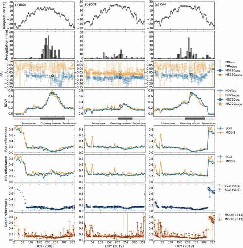
Figure 8. Comparison of NDVI_SGLI with NDVI_MODIS on (a) the relationship between NDVI and the ratio of the soil surface to vegetation cover in wet and dry soils (b) the difference in NDVI on dry and wet soils. The simulation was conducted using the spectral reflectance of grass, wet soil, and dry soil, which are described in Fig. 4.

Figure 9. Comparison of the in-situ PRI_SGLI and the satellite PRI_SGLI at all sites. The satellite PRI was taken on the closest sunny day to the day of the in-situ observation. For the DGT site, the satellite PRI of two days (the closest sunny day: 2019-08-10 and the same day with the in-situ observation but cloudy: 2019-08-09) was demonstrated. The RMSE for all data was calculated using 1) BGN, DGT (satellite data on 2019-08-09), and KYM data and 2) BGN, DGT (satellite data on 2019-08-10), and KYM data.

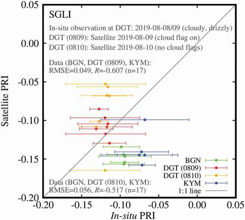
Figure 10. Relationship between PRI_SGLI and the ratio of the soil surface to vegetation cover on dry and wet soils. The simulation was conducted using the spectral reflectance of grass, wet soil, and dry soil, which are described in Fig. 4.

Figure 11. Spatial distribution of PRI derived from SGLI in (a) the area including three study sites on (b) August 23, 2018 (the peak of greenness), and (c) October 03, 2018 (the end of the growing season). (d) Subtraction of (b) from (c).

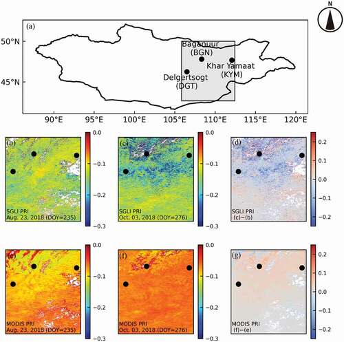
Figure 12. Comparison of the band reflectance between the SGLI (satellite data) and the MS-720 spectroradiometer (in-situ data) at the (a) BGN, (b) DGT, and (c) KYM sites. The daily SGLI band reflectance data were taken on the closest sunny day to the day of the in-situ observation. For the DGT site, the SGLI data of two days (the closest sunny day: 2019-08-10 and the same day with the in-situ observation but cloudy: 2019-08-09) was demonstrated. The bars for the band reflectance and the VI denote the standard error of the mean and the uncertainty of the mean (calculated by Eq. 6(6) $\sigma =\frac{2y}{{\left(x+y\right)}^2}\sqrt{{{\sigma }_x}^2+{{\sigma }_y}^2.}$(6) ) within the target area at each observation site, respectively. The *, **, and *** indicate p-values less than 0.05, 0.01, and 0.001, respectively (Welch’s t-test).

Figure 13. Dates of phenological events (DPE) detected from the in-situ observation (time-lapse camera) and the satellite time-series NDVI at the BGN site in 2018. The time-lapse camera images, shown above the graphs, were taken on the DPE detected from three sources (camera, NDVI_SGLI, and NDVI_MODIS). The blue line denotes the NDVI_SGLI, and the orange line is the NDVI_MODIS.

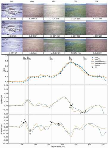
Figure 14. Comparison of the annual maximum NDVI of SGLI and MODIS in 2019 in each natural zone [delineated in (a)] of Mongolia (Dash, 2005): (b) the entire of Mongolia, (c) mountain-taiga and forest-steppe, (f) steppe, (e) semi-desert, and (f) desert. The colour bar denotes the number of pixels. The dashed line in a scatter diagram is the 1:1 line. (g)–(j) Images of typical vegetation cover of each natural zones.

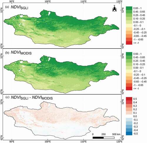
Figure 15. Spatial distributions of the annual maxima of (a) NDVI_SGLI, (b) NDVI_MODIS, and (c) the difference in 2019.

Nasahara, K. N., and S. Nagai. 2015. “Development of an in situ Observation Network for Terrestrial Ecological Remote Sensing: The Phenological Eyes Network (PEN).” Ecological Research 30 (2): 211–223. doi:10.1007/s11284-014-1239-x.

 Web of Science ®Google Scholar

Baumgardner, M. F., L. F. Silva, L. L. Biehl, and E. R. Stoner. 1986. “Reflectance Properties of Soils.” Advances in Agronomy 38: 1–44.

 Web of Science ®Google Scholar

Dash, D. Natural Zone. 2005. Shapefile. Available online: https://eic.mn/geodata/download.php (accessed on May 10, 2020).

 Google Scholar

Data availability statement

The observed spectral data that support the findings of this study are available from the corresponding author, Akitsu T.K., upon reasonable request.