SAR image edge detection: review and benchmark experiments

Figures & data

Figure 1. A) Ratio-based edge detector using σ_hh (L-band). Credits: (Schou et al. 2003) b) RBED edge detector. Credits: (Wei and Feng 2015). c) Multiscale edge detector. Credits: (Xiang et al. 2017a).

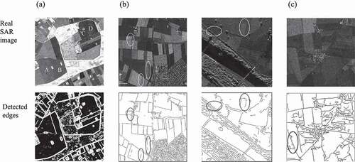
Figure 2. Examples of synthetic images of simulated simple scenarios. a) Wei and Feng (2015) b) Zhan et al. (2013) c) Xiang et al. (2017b).

Figure 3. A) Denoised with SAR-BM3D. Credits: (Parrilli et al. 2011). b) Denoised with soft thresholding. Credits: (Achim et al. 2003). c) Denoised with SAR-CNN. Credits: (Molini et al. 2020).

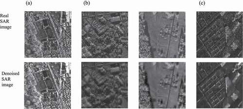
Figure 4. Difference in first and second derivatives-based edge detection. f indicates the image intensity.

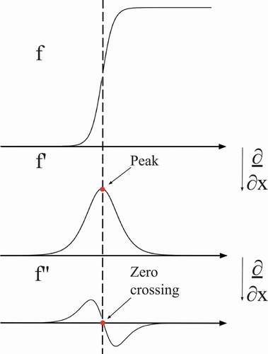
Figure 5. First order derivatives-based edge detection workflow.

Figure 6. Examples of directional filters. α is measured counterclockwise from the horizontal axis. Credits: Schowengerdt (2007).

Figure 7. Example of the real parts of the Gabor filters with different orientations and frequencies to capture various patterns. These filters are also used to create one of our filter banks.

Figure 8. Subpixel edge detection where edges are precisely located inside the pixels. Credits: (Trujillo-Pino et al. 2013).

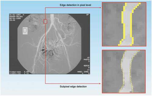
Figure 9. Subpixel edge detection algorithm based on partial area effect. a) Input image; b) Smoothed image; c) Detecting edge pixels; d) a synthetic 9×3 subimage is created from the features of each edge pixel; e) Subimages are combined to achieve a complete restored image. Credits: (Trujillo-Pino et al. 2013).

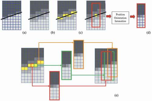
Figure 10. Scheme of the ROA method. Credits: Dellinger et al. (2015).

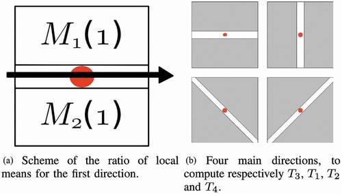
Figure 11. Difference between (a) rectangle bi-windows and (b) GGS bi-windows at orientation ^π . Credits: Shui and Cheng (2012).

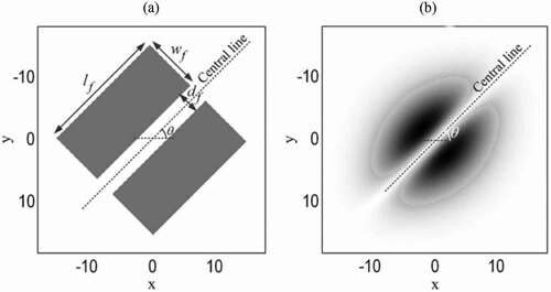
Figure 12. (a) Circular window with 4 pixel radius, (b) prototype pattern (bar) for RUSTICO, (c) positions of local differences of the Gaussians’ maxima along with concentric circles. Credits: Li et al. (2022).

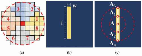
Figure 13. Fundamental edge detection steps.

Figure 14. Sample images from the BSDS500-speckled dataset.

Table 1. Evaluation of various denoising methods over the entire BSDS500-speckled dataset.

Method	MSE$\downarrow$	PSNR$\uparrow$	SSIM$\uparrow$
SARBLF (N=2, gs=2.2, gr=1.33)	0.0109	28.8672	0.7211
SARBLF (N=3, gs=2.2, gr=1.33)	0.0105	28.8904	0.7212
SARBLF (N=4, gs=2.2, gr=1.33)	0.0115	28.8321	0.7076
SARBLF (N=3, gs=2.8, gr=1.4)	0.0121	28.7958	0.7023
Anisotropic Diffusion (N=1)	0.0793	27.8338	0.4095
Anisotropic Diffusion (N=2)	0.0596	27.9018	0.4808
Anisotropic Diffusion (N=10)	0.0229	28.2714	0.6460
Anisotropic Diffusion (N=15)	0.0185	28.3742	0.6667
NLMD ($\sigma$=0.5)	0.0748	27.9419	0.5385
BM3D ($\sigma$=0.5)	0.0550	27.9572	0.6023

Figure 15. Qualitative evaluation results of the denoising methods.

Table 2. Evaluation of the first-order derivatives-based edge detectors.

Setup	ACC$\uparrow$	F1$\uparrow$	PPV$\uparrow$	FM$\uparrow$
Farid	0.7483	0.3581	0.3300	0.3768
Prewitt	0.7168	0.3576	0.2972	0.3823
Sobel	0.7259	0.3573	0.3024	0.3795
Scharr	0.7606	0.3563	0.3296	0.3715
Roberts	0.7530	0.3498	0.3192	0.3665
Frei-Chen	0.5540	0.3053	0.2102	0.3584

Figure 16. ROC curves of the first-order derivatives-based edge detectors.

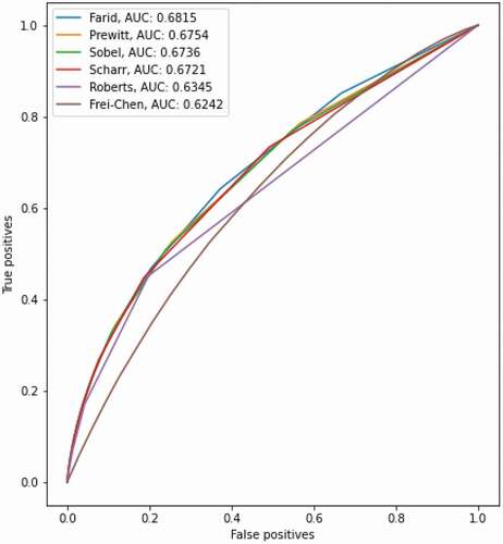
Table 3. Evaluation of the different parameters for LoG.

Setup	ACC$\uparrow$	F1$\uparrow$	PPV$\uparrow$	FM$\uparrow$
$\sigma =1.0$	0.6536	0.1894	0.1598	0.2009
$\sigma =1.4$	0.6745	0.1852	0.1632	0.1943
$\sigma =2.0$	0.6988	0.1796	0.1684	0.1866
$\sigma =2.7$	0.7225	0.1734	0.1753	0.1791
$\sigma =3.0$	0.7312	0.1708	0.1783	0.1762

Table 4. Evaluation of the different parameters for DoG. Ratio indicates the size ratio of the kernels.

Setup	ACC$\uparrow$	F1$\uparrow$	PPV$\uparrow$	FM$\uparrow$
${\sigma }_1=1.0$ $|$ ratio = 4	0.7152	0.1757	0.1737	0.1818
${\sigma }_1=1.0$ $|$ ratio = 5	0.7273	0.1725	0.1783	0.1783
${\sigma }_1=1.4$ $|$ ratio = 4	0.7388	0.1690	0.1830	0.1746
${\sigma }_1=1.4$ $|$ ratio = 5	0.7495	0.1655	0.1888	0.1714
${\sigma }_1=2.0$ $|$ ratio = 4	0.7631	0.1596	0.1961	0.1663
${\sigma }_1=2.0$ $|$ ratio = 5	0.7716	0.1555	0.2027	0.1634
${\sigma }_1=2.7$ $|$ ratio = 4	0.7815	0.1486	0.2089	0.1580
${\sigma }_1=2.7$ $|$ ratio = 5	0.7882	0.1441	0.2159	0.1552
${\sigma }_1=3.0$ $|$ ratio = 4	0.7874	0.1440	0.2136	0.1547
${\sigma }_1=3.0$ $|$ ratio = 5	0.7935	0.1394	0.2208	0.1519

Table 5. Evaluation of Canny edge detection for different sigma options and threshold ratios.

Setup	ACC$\uparrow$	F1$\uparrow$	PPV$\uparrow$	FM$\uparrow$
$\sigma =1.0$ $|$ ratio = 2	0.7885	0.1829	0.2512	0.1930
$\sigma =1.0$ $|$ ratio = 3	0.7827	0.1826	0.2409	0.1914
$\sigma =1.4$ $|$ ratio = 2	0.7972	0.1793	0.2618	0.1913
$\sigma =1.4$ $|$ ratio = 3	0.7920	0.1791	0.2513	0.1896
$\sigma =2.0$ $|$ ratio = 2	0.8047	0.1736	0.2734	0.1882
$\sigma =2.0$ $|$ ratio = 3	0.8008	0.1735	0.2637	0.1866
$\sigma =2.7$ $|$ ratio = 2	0.8105	0.1664	0.2833	0.1839
$\sigma =2.7$ $|$ ratio = 3	0.8079	0.1665	0.2751	0.1826
$\sigma =3.0$ $|$ ratio = 2	0.7963	0.1632	0.2438	0.1749
$\sigma =3.0$ $|$ ratio = 3	0.8103	0.1632	0.2792	0.1806

Table 6. Evaluation of Gabor edge detection for different scales (S) and orientations (O).

Setup	ACC$\uparrow$	F1$\uparrow$	PPV$\uparrow$	FM$\uparrow$
$S=2$ $|$ $O=3$	0.6208	0.3092	0.2328	0.3478
$S=3$ $|$ $O=5$	0.6113	0.3210	0.2381	0.3650
$S=4$ $|$ $O=6$	0.6147	0.3294	0.2443	0.3749
$S=5$ $|$ $O=8$	0.6440	0.3404	0.2584	0.3819

Figure 17. ROC curves of the Gabor filter-banks.

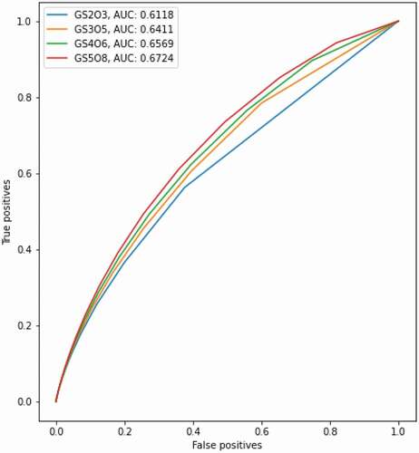
Table 7. Evaluation of different number of clusters for K-means-based edge detection.

Setup	ACC$\uparrow$	F1$\uparrow$	PPV$\uparrow$	FM$\uparrow$
$k=3$	0.7636	0.2747	0.2892	0.2835
$k=4$	0.7200	0.2966	0.2609	0.3108
$k=5$	0.6809	0.3094	0.2467	0.3329

Figure 18. ROC curves of the K-means clustering-based edge detection.

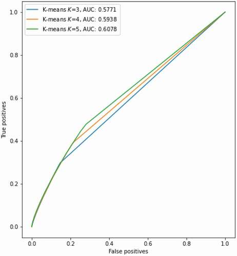
Figure 19. ROC curve of the 2D Discrete Wavelet Transformation-based edge detection.

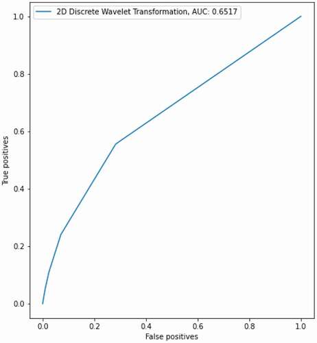
Table 8. Evaluation of 2D discrete wavelet transformation-based edge detection.

Setup	ACC$\uparrow$	F1$\uparrow$	PPV$\uparrow$	FM$\uparrow$
2D Discrete Wavelet	0.7000	0.3557	0.2855	0.3852

Table 9. Evaluation of different iterations for the subpixel-based edge detection method.

Setup	ACC$\uparrow$	F1$\uparrow$	PPV$\uparrow$	FM$\uparrow$
$iter=1$	0.7330	0.1581	0.1701	0.1634
$iter=2$	0.7005	0.1754	0.1650	0.1820
$iter=3$	0.6963	0.1772	0.1643	0.1840

Figure 20. ROC curves of Touzi for different radius values.

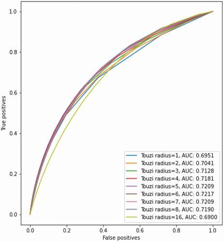
Table 10. Evaluation of different parameters for Touzi.

Setup	ACC$\uparrow$	F1$\uparrow$	PPV$\uparrow$	FM$\uparrow$
$radius=1$	0.7582	0.3739	0.3366	0.3922
$radius=2$	0.7267	0.3788	0.3159	0.4051
$radius=3$	0.7515	0.3866	0.3351	0.4071
$radius=4$	0.7304	0.3899	0.3186	0.4162
$radius=5$	0.7132	0.3892	0.3067	0.4204
$radius=6$	0.7438	0.3877	0.3254	0.4099
$radius=7$	0.7319	0.3852	0.3150	0.4103
$radius=8$	0.7208	0.3817	0.3057	0.4094
$radius=16$	0.6492	0.3510	0.2562	0.3932

Table 11. Evaluation of different parameters for GR.

Setup	ACC$\uparrow$	F1$\uparrow$	PPV$\uparrow$	FM$\uparrow$
$\alpha =1$	0.6956	0.3365	0.3007	0.3736
$\alpha =2$	0.7319	0.3610	0.3198	0.3885
$\alpha =3$	0.7088	0.3705	0.3039	0.4032
$\alpha =4$	0.6867	0.3708	0.2893	0.4087
$\alpha =5$	0.6704	0.3677	0.2790	0.4092
$\alpha =6$	0.6551	0.3633	0.2699	0.4081

Figure 21. ROC curves of GR for different sigma values.

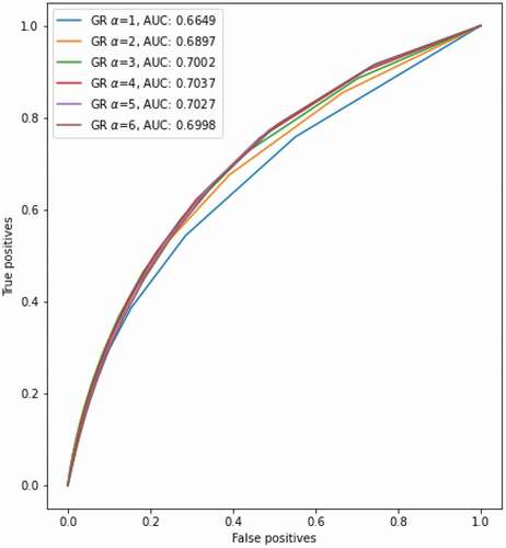
Table 12. Evaluation of different parameters for the Gaussian-Gamma-shaped bi-windows.

Setup	ACC$\uparrow$	F1$\uparrow$	PPV$\uparrow$	FM$\uparrow$
$\alpha =2|w=7.0|l=6.5$	0.8109	0.1453	0.2675	0.1642
$\alpha =2|w=7.0|l=7.0$	0.8111	0.1458	0.2689	0.1648
$\alpha =2|w=9.0|l=6.5$	0.8150	0.1372	0.2746	0.1590
$\alpha =2|w=9.0|l=7.0$	0.8149	0.1378	0.2749	0.1594
$\alpha =3|w=7.0|l=6.5$	0.8084	0.1420	0.2544	0.1593
$\alpha =3|w=7.0|l=7.0$	0.8086	0.1426	0.2554	0.1599
$\alpha =3|w=9.0|l=6.5$	0.8147	0.1324	0.2666	0.1537
$\alpha =3|w=9.0|l=7.0$	0.8144	0.1328	0.2661	0.1539
$\alpha =4|w=7.0|l=6.5$	0.8199	0.1384	0.3028	0.1649
$\alpha =4|w=7.0|l=7.0$	0.8197	0.1387	0.3026	0.1651
$\alpha =4|w=9.0|l=6.5$	0.8156	0.1273	0.2643	0.1492
$\alpha =4|w=9.0|l=7.0$	0.8154	0.1276	0.2638	0.1493

Table 13. Evaluation of different parameters for ROLSS RUSTICO.

Setup	ACC$\uparrow$	F1$\uparrow$	PPV$\uparrow$	FM$\uparrow$
$\xi =1.0|\lambda =0.5$	0.7718	0.1475	0.2352	0.1644
$\xi =1.0|\lambda =1.0$	0.7700	0.1489	0.2355	0.1658
$\xi =1.0|\lambda =2.0$	0.7681	0.1529	0.2366	0.1696
$\xi =1.0|\lambda =3.0$	0.7607	0.1607	0.2324	0.1763
$\xi =1.5|\lambda =0.5$	0.7727	0.1479	0.2359	0.1647
$\xi =1.5|\lambda =1.0$	0.7700	0.1496	0.2361	0.1665
$\xi =1.5|\lambda =2.0$	0.7676	0.1544	0.2370	0.1710
$\xi =1.5|\lambda =3.0$	0.7590	0.1634	0.2319	0.1787
$\xi =2.0|\lambda =0.5$	0.7736	0.1482	0.2365	0.1650
$\xi =2.0|\lambda =1.0$	0.7701	0.1501	0.2365	0.1671
$\xi =2.0|\lambda =2.0$	0.7672	0.1554	0.2373	0.1720
$\xi =2.0|\lambda =3.0$	0.7578	0.1649	0.2315	0.1801

Table 14. Evaluation of different parameters for SAR-Shearlet, where $l$ denotes the effective support length of the Mexican hat wavelet.

Setup	ACC$\uparrow$	F1$\uparrow$	PPV$\uparrow$	FM$\uparrow$
$Shearlevel=2|scales=2|l=1/2$	0.7660	0.2836	0.2960	0.2963
$Shearlevel=2|scales=3|l=1/2$	0.1595	0.2680	0.1595	0.3876
$Shearlevel=2|scales=2|l=1/7$	0.1595	0.2680	0.1595	0.3876
$Shearlevel=2|scales=3|l=1/7$	0.1595	0.2680	0.1595	0.3876
$Shearlevel=3|scales=2|l=1/7$	0.1595	0.2680	0.1595	0.3876
$Shearlevel=3|scales=3|l=1/7$	0.1595	0.2680	0.1595	0.3876
$Shearlevel=4|scales=2|l=1/7$	0.1595	0.2680	0.1595	0.3876
$Shearlevel=4|scales=3|l=1/7$	0.1595	0.2680	0.1595	0.3876

Figure 22. ROC curves of SAR-Shearlet for different parameters.

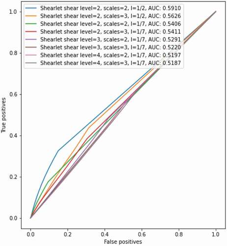
Table 15. Evaluation of the fusion schemes for combining the SAR-specific Touzi and optical Farid methods.

Setup	ACC$\uparrow$	F1$\uparrow$	PPV$\uparrow$	FM$\uparrow$
Single voting	0.6816	0.3739	0.2816	0.4117
Complete agreement	0.8104	0.3735	0.4143	0.3847
Touzi($r=6$)	0.7438	0.3877	0.3254	0.4099
Farid	0.7483	0.3581	0.3300	0.3768

Table 16. Evaluation of the fusing schemes for combining the ROA-based Touzi and ROEWA-based GR.

Setup	ACC$\uparrow$	F1$\uparrow$	PPV$\uparrow$	FM$\uparrow$
Single voting	0.6803	0.3793	0.2891	0.4186
Complete agreement	0.7502	0.3792	0.3259	0.4001
Touzi($r=6$)	0.7438	0.3877	0.3254	0.4099
GR($\alpha =4$)	0.6867	0.3708	0.2893	0.4087

Table 17. Evaluation of the gradient magnitude fusion for the SAR-specific Touzi and non-SAR Farid method.

Setup	ACC$\uparrow$	F1$\uparrow$	PPV$\uparrow$	FM$\uparrow$
Gradient Fusion	0.7481	0.3933	0.3313	0.4149
Touzi($r=6$)	0.7438	0.3877	0.3254	0.4099
Farid	0.7483	0.3581	0.3300	0.3768

Table 18. Evaluation of the gradient magnitude fusion for combining the ROA-based Touzi and ROEWA-based GR.

Setup	ACC$\uparrow$	F1$\uparrow$	PPV$\uparrow$	FM$\uparrow$
Gradient Fusion	0.7237	0.3854	0.3108	0.4133
Touzi($r=6$)	0.7438	0.3877	0.3254	0.4099
GR($\alpha =4$)	0.6867	0.3708	0.2893	0.4087

Figure 23. ROC curve of gradient fusion.

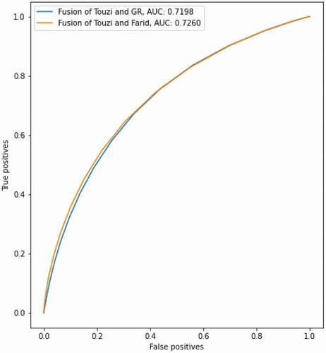
Table 19. Overview of the best performing methods over the training set, ranked by F1-score.

Algorithm	ACC$\uparrow$	F1$\uparrow$	PPV$\uparrow$	FM$\uparrow$
GGS bi-windows ($\alpha =2|w=7|l=7$)	0.8111	0.1458	0.2689	0.1648
ROLSS RUSTICO ($\xi =2|\lambda =3$)	0.7578	0.1649	0.2315	0.1801
DoG(${\sigma }_1=1.0$ $|$ ratio = 4)	0.7152	0.1757	0.1737	0.1818
Subpixel ($iter=3$)	0.6963	0.1772	0.1643	0.1840
Canny ($\sigma =1.0$ $|$ ratio = 2)	0.7885	0.1829	0.2512	0.1930
LoG ($\sigma =1.0$)	0.6536	0.1894	0.1598	0.2009
Shearlet $(Shearlevel=2|scales=2|l=1/2)$	0.7660	0.2836	0.2960	0.2963
Frei-Chen	0.5540	0.3053	0.2102	0.3584
K-means ($k=5$)	0.6809	0.3094	0.2467	0.3329
Gabor (GS5O8)	0.6440	0.3404	0.2584	0.3819
Roberts	0.7530	0.3498	0.3192	0.3665
2D Discrete Wavelet	0.7000	0.3557	0.2855	0.3852
Scharr	0.7606	0.3563	0.3296	0.3715
Sobel	0.7259	0.3573	0.3024	0.3795
Prewitt	0.7168	0.3576	0.2972	0.3823
Farid	0.7483	0.3581	0.3300	0.3768
GR ($\alpha =4$)	0.6867	0.3708	0.2893	0.4087
Binary Fusion	0.8104	0.3735	0.4143	0.3847
Touzi ($r=6$)	0.7438	0.3877	0.3254	0.4099
Gradient Fusion	0.7481	0.3933	0.3313	0.4149

Table 20. BSDS500-speckled Benchmark. The rows are sorted by ODS F1. The best results are highlighted in bold, while the second best results are underlined.

Algorithm	OIS (F1)	ODS (F1)	AP	Threshold
Subpixel ($iter=3$)	0.3019	0.3013	0.1775	0.1290
LoG ($\sigma =1.0$)	0.3333	0.3329	0.1999	0.7097
DoG (${\sigma }_1=1.0$ $|$ ratio = 4)	0.3902	0.3899	0.2453	0.3871
GS5O8	0.4407	0.3965	0.3660	0.1613
ROLSS RUSTICO ($\xi =2|\lambda =3$)	0.4194	0.4190	0.3563	0.0645
K-means ($k=5$)	0.5349	0.4778	0.3336	0.1936
Canny ($\sigma =1.0$ $|$ ratio = 2)	0.4838	0.4835	0.3467	0.6774
Gradient Fusion	0.4859	0.4856	0.3517	0.0968
Shearlet $(Shearlevel=2|scales=2|l=1/2)$	0.5132	0.5022	0.4293	0.0645
2D Discrete Wavelet	0.5428	0.5303	0.5278	0.0645
Farid	0.5599	0.5303	0.4913	0.1613
GGS bi-windows ($\alpha =2|w=7|l=7$)	0.5332	0.5329	0.3988	0.3226
Roberts	0.5470	0.5334	0.5254	0.0645
Sobel	0.5547	0.5350	0.4983	0.1290
Prewitt	0.5550	0.5353	0.4815	0.1290
Scharr	0.5525	0.5356	0.4467	0.0968
Frei-Chen	0.5481	0.5429	0.4430	0.9032
GR ($\alpha =4$)	0.5807	0.5437	0.5194	0.1613
Binary Fusion	0.5583	0.5581	0.6211	0.8710
Touzi ($r=6$)	0.5922	0.5672	0.5437	0.2903
Gradient Fusion	0.6015	0.5820	0.5493	0.4516
GRHED($\alpha =2,3,4,5$) (Liu et al. 2020)	0.6119	0.6115	0.6450	0.7419

Table 21. BSDS500-speckled Noisy Benchmark. The rows are sorted by ODS F1. The best results are highlighted in bold, while the second best results are underlined.

Algorithm	OIS (F1)	ODS (F1)	AP	Threshold
GGS bi-windows ($\alpha =2|w=7|l=7$)	0.3622	0.3618	0.2217	0.4194
ROLSS RUSTICO ($\xi =2|\lambda =3$)	0.4142	0.4137	0.3401	0.3226
Shearlet $(Shearlevel=2|scales=2|l=1/2)$	0.5130	0.4950	0.4000	0.3226
Binary Fusion	0.5403	0.5396	0.4252	0.0323
GR ($\alpha =4$)	0.5893	0.5459	0.4744	0.1935
Gradient Fusion	0.5719	0.5533	0.5049	0.5806
Touzi ($r=6$)	0.5928	0.5703	0.5068	0.3871
GRHED ($\alpha =2,3,4,5$) (Liu et al. 2020)	0.6510	0.6505	0.5863	0.2903

Figure 24. A) Original clean Sentinel-1 Lelystad image. Credits image: Dalsasso et al. (2021) b) Pseudo ground-truth. Credits image: Liu et al., (2020) c) 1-look speckled image. d) Denoised 1-look image.

Table 22. The performances of different methods on the Sentinel-1 Lelystad, ordered by F1 score.

Algorithm	ACC$\uparrow$	F1$\uparrow$	PPV$\uparrow$	FM$\uparrow$	Threshold
ROLSS RUSTICO ($\xi =2|\lambda =3$)	0.9046	0.0462	0.0504	0.0463	0.05
Subpixel	0.7265	0.1036	0.0630	0.1355	0.0
LoG ($\sigma =1.0$)	0.6987	0.1062	0.0632	0.1445	-
DoG (${\sigma }_1=1.0$ $|$ ratio = 4)	0.7749	0.1143	0.0726	0.1395	-
Shearlet $(Shearlevel=2|scales=2|l=1/2)$	0.7944	0.1710	0.1094	0.2069	0.05
GS5O8	0.9066	0.1760	0.1686	0.1762	0.2
Frei-Chen	0.6904	0.1971	0.1147	0.2836	0.45
GGS bi-windows ($\alpha =2|w=7|l=7$)	0.9142	0.1972	0.1998	0.1972	0.15
K-means ($k=5$)	0.7700	0.2075	0.1275	0.2662	0.05
Canny ($\sigma =1.0$ $|$ ratio = 2)	0.9154	0.2325	0.2287	0.2325	0.15
Wavelet	0.7814	0.2572	0.1576	0.3318	0.05
GR ($\alpha =4$)	0.7972	0.2635	0.1640	0.3314	0.15
GRHED ($\alpha =2,3,4,5$) (Liu et al. 2020)	0.9370	0.2817	0.3681	0.2898	0.5516
Touzi ($r=6$)	0.8625	0.2896	0.2011	0.3226	0.3
Prewitt	0.8602	0.3034	0.2078	0.3417	0.1
Roberts	0.8791	0.3057	0.2219	0.3302	0.05
Farid	0.9184	0.3060	0.2839	0.3069	0.15
Binary Fusion	0.9260	0.3064	0.3111	0.3065	-
Sobel	0.8742	0.3101	0.2207	0.3393	0.1
Gradient Fusion	0.8822	0.3120	0.2282	0.3354	0.45
Scharr	0.8847	0.3150	0.2323	0.3371	0.1

Figure 25. Edge detection performances on a single look Sentinel-1 image of Lelystad.

Table 23. Run times (measured in seconds) of the algorithms for SAR image evaluations.¹¹.

Algorithm	Runtime (Odessa) $\downarrow$	Runtime (Lelystad) $\downarrow$
Subpixel	1459.92	538.62
GS5O8	979.05	541.69
GRHED	105.97	65.13
ROLSS RUSTICO	52.07	23.81
Shearlet	37.05	13.34
DoG	7.06	5.09
LoG	6.43	4.77
K-means	5.43	5.19
Gradient Fusion	3.29	2.01
GGS bi-windows	2.03	0.82
Canny	1.88	0.54
GR	1.80	0.81
Binary Fusion	1.68	1.26
Touzi	0.95	0.89
Frei-Chen	0.60	0.31
Farid	0.33	0.17
Wavelet	0.16	0.21
Prewitt	0.16	0.09
Sobel	0.16	0.09
Scharr	0.16	0.09
Roberts	0.13	0.07

Figure 26. A single look TerraSAR-X image of Texas, USA, around the Winkler County Sinkhole #2 near Odessa. Credits: © DLR e.V. 2022 and © Airbus Defence and Space GmbH 2022. a) Original noisy image. b) Denoised with SARBLF.

Figure 27. Edge detection performances on a TerraSAR-X image of Texas, USA, around the Winkler County Sinkhole #2 near Odessa. Credits: © DLR e.V. 2022 and © Airbus Defence and Space GmbH 2022.

Figure 28. Sentinel-1 image of Texas, USA, captured around Red Bluff Reservoir on the Pecos River near Reeves County with different polarizations. a) Sigma0 VH b) Sigma0 VV. Both images are denoised by SAR- BLF. Credits: Copernicus Sentinel data 2022.

Table 24. Matching consistency of different algorithms over different polarizations (VV and VH) of the same area of 1900 by 7200 pixels (13.68 million pixels), ordered by MEP.

Algorithm	Matching Edge Percentage (MEP) $\uparrow$	Matching Pixel Percentage (MPP) $\uparrow$
Binary Fusion	0.01%	95.32%
Farid	0.02%	93.65%
Sobel	0.02%	97.54%
Scharr	0.03%	99.19%
Prewitt	0.03%	96.60%
Wavelet	0.06%	96.72%
Roberts	0.20%	99.43%
GS5O8	1.18%	94.65%
DoG	21.54%	70.22%
GGS bi-windows	23.08%	99.38%
Subpixel	26.03%	62.66%
LoG	26.99%	63.11%
Canny	28.98%	99.38%
ROLSS RUSTICO	29.54%	62.78%
Frei-Chen	29.88%	84.54%
Gradient Fusion	31.24%	81.43%
Touzi	37.10%	92.11%
K-means	42.07%	55.82%
GR	48.06%	67.94%
GRHED	66.69%	99.89%
Shearlet	74.64%	98.71%

Schou, J., H. Skriver, A. A. Nielsen, and K. Conradsen. 2003. “CFAR Edge Detector for Polarimetric SAR Images.” IEEE Transactions on Geoscience and Remote Sensing 41 (1): 20–32. doi:10.1109/TGRS.2002.808063.

 Web of Science ®Google Scholar

Wei, Q. R., and D. Z. Feng. 2015. “An Efficient SAR Edge Detector with a Lower False Positive Rate.” International Journal of Remote Sensing 36 (14): 3773–3797.

 Web of Science ®Google Scholar

Xiang, Y., F. Wang, L. Wan, and H. You. 2017a. “An Advanced Multiscale Edge Detector Based on Gabor Filters for SAR Imagery.” IEEE Geoscience and Remote Sensing Letters 14 (9): 1522–1526. doi:10.1109/LGRS.2017.2720684.

 Web of Science ®Google Scholar

Zhan, Y., H. You, and C. Fuqing. 2013. “Bayesian Edge Detector for SAR Imagery Using Discontinuity-Adaptive Markov Random Field Modeling.” Chinese Journal of Aeronautics 26 (6): 1534–1543. doi:10.1016/j.cja.2013.04.059.

 Web of Science ®Google Scholar

Xiang, Y., F. Wang, L. Wan, and H. You. 2017b. “SAR-PC: Edge Detection in Sar Images via an Advanced Phase Congruency Model.” Remote Sensing 9 (3): 209. doi:10.3390/rs9030209.

 Web of Science ®Google Scholar

Parrilli, S., M. Poderico, C. V. Angelino, and L. Verdoliva. 2011. “A Nonlocal SAR Image Denoising Algorithm Based on LLMMSE Wavelet Shrinkage.” IEEE Transactions on Geoscience and Remote Sensing 50 (2): 606–616.

 Web of Science ®Google Scholar

Achim, A., P. Tsakalides, and A. Bezerianos. 2003. “SAR Image Denoising via Bayesian Wavelet Shrinkage Based on Heavy-Tailed Modeling.” IEEE Transactions on Geoscience and Remote Sensing 41 (8): 1773–1784. doi:10.1109/TGRS.2003.813488.

 Web of Science ®Google Scholar

Molini, A. B., D. Valsesia, G. Fracastoro, and E. Magli. 2020. “Towards Deep Unsupervised SAR Despeckling with Blind-Spot Convolutional Neural Networks.” In IEEE International Geoscience and Remote Sensing Symposium, Waikoloa, HI, USA, 2507–2510. IEEE.

 Google Scholar

Schowengerdt, R. A. 2007. ”Chapter 6 - Spatial Transforms”. In Remote Sensing (Third Edition), 3rd ed. edited by R. A. Schowengerdt, 229–283. Burlington: Academic Press.

 Google Scholar

Trujillo-Pino, A., K. Krissian, M. Aleman-Flores, and D. Santana-Cedres. 2013. “Accurate Subpixel Edge Location Based on Partial Area Effect.” Image and Vision Computing 31 (1): 72–90. doi:10.1016/j.imavis.2012.10.005.

 Web of Science ®Google Scholar

Dellinger, F., J. Delon, Y. Gousseau, J. Michel, and F. Tupin. 2015. “SAR-SIFT: A SIFT-Like Algorithm for SAR Images.” IEEE Transactions on Geoscience and Remote Sensing 53 (1): 453–466. doi:10.1109/TGRS.2014.2323552.

 Web of Science ®Google Scholar

Shui, P. L., and D. Cheng. 2012. “Edge Detector of SAR Images Using Gaussian-Gamma-Shaped Bi-Windows.” IEEE Geoscience and Remote Sensing Letters 9 (5): 846–850.

 Web of Science ®Google Scholar

Li, J., W. Yu, Z. Wang, Y. Luo, and Z. Yu. 2022. “A Robust Statistic-Aided Edge Detector for SAR Images Based on RUSTICO.” Electronics Letters 58 (10): 393–395. doi:10.1049/ell2.12473.

 Web of Science ®Google Scholar

Liu, C., F. Tupin, and Y. Gousseau. 2020. “Training CNNs on Speckled Optical Dataset for Edge Detection in SAR Images.” ISPRS Journal of Photogrammetry and Remote Sensing 170: 88–102. doi:10.1016/j.isprsjprs.2020.09.018.

 Web of Science ®Google Scholar

Dalsasso, E., L. Denis, and F. Tupin. 2021. “SAR2SAR: A Semi-Supervised Despeckling Algorithm for SAR Images.” IEEE Journal of Selected Topics in Applied Earth Observations and Remote Sensing 14: 4321–4329. doi:10.1109/JSTARS.2021.3071864.

 Web of Science ®Google Scholar

Data availability statement

The data that support the findings of this study are available at https://github.com/ChenguangTelecom/GRHED, and the benchmark suite is available at https://github.com/readmees/SAR_edge_benchmark.