Figures & data
Figure 1. Map of the Kathmandu Valley. The black contour is the valley watershed. The dark blue network is the major rivers in the valley. The sediment thickness is up to 500 m. The black dashed line is a proximate location of the schematic cross-section shown in Figure 2. The inset location map is made with GeoMapApp (www.geomapapp.org) (Ryan et al. Citation2009). The sediment thickness data are from JICA (Citation2018). The river network shapefile is from Thapa et al. (Citation2022), which is sourced from the department of survey in Nepal.
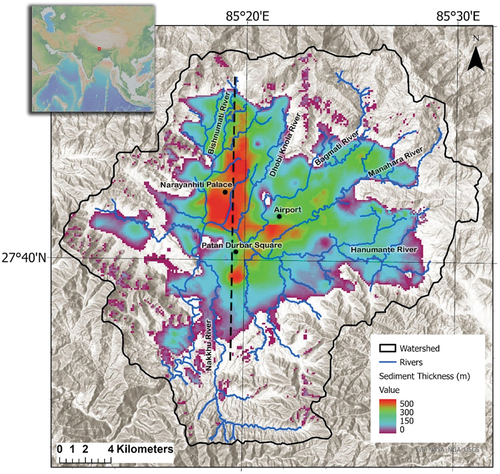
Figure 2. North-South generalized representative cross-section schematic model of Kathmandu Valley. An approximate location of the cross-section is shown in Figure 1 as a black dashed line. The basin stratigraphy is classified into five distinct stratigraphic units. Sa represents the shallow aquifer, SG represents the deep aquifer, CS represents the aquitard and CG with mixed aquifer characteristics. BR is the basement made up of metasandstone, phyllite, schist and quartzite. The maximum thickness of the aquitard is ~200 m and similarly the maximum thickness of the deep aquifer is ~300 m around the central part of the basin. The central part of the basin is the region where the maximum subsidence is observed. The shallow aquifer is recharged during each monsoon season directly from the precipitation. The chances of vertical recharge for the deep aquifer from precipitation is negligible due to the presence of a thick aquitard above it. Infiltration from the top sandy layer and bed rock aquifer (weathered gneiss, metasandstone, limestone) in the marginal part may have some contribution to the deep aquifer. Note that the maximum variation in thickness is controlled by the lower sandy gravel unit (SG), which represents the deep aquifer.
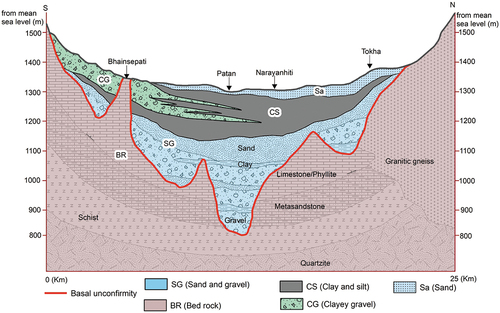
Figure 3. The network of all available pairs of interferograms. The y-axis is the perpendicular baseline, versus acquisition dates on the x-axis. The perpendicular baseline is the distance between the satellite orbits when the satellite revisits the ‘same location’. Each blue line connects two SAR images for interferograms. All the SAR images are co-registered with the master reference SAR image (red circle, 2016/09/14 for the descending and 2016/09/06 for the ascending).
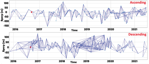
Figure 4. The SBAS-InSAR results from (a) 2015/10/06 to 2021/07/06 for the ascending and (b) 2015/11/07 to 2021/07/02 for the descending. The overall velocities from the ascending and descending are similar. (c) The vertical velocities are from 2015/11/07 to 2021/07/02. (d) In the horizontal (EW) motion map, positive values mean eastward displacement. The 10 coloured triangles in (a) are the locations for the time-series analysis. The reference point in (a) is the black star located in the south of the Kathmandu Valley. The yellow square in (a) is the GPS location.
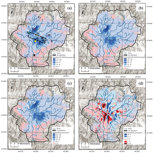
Figure 5. Maps of uncertainty in the subsidence rates. (a) Ascending velocity standard deviation. (b) descending velocity standard deviation. InSAR LOS velocity standard deviation ranges 0–1 mm year−1. The relative high values in velocity standard deviation could be caused by relatively high uncertainty values, or a non-linear signal in the time-series.
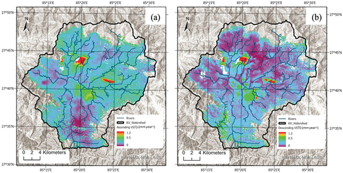
Figure 6. Comparison of the GPS, ascending and descending SBAS-InSAR time-series at the NAST-GPS location. The InSAR derived time-series at the GPS location closely agrees with the time series measured by GPS. The NGL has GPS data available up to year 2020 at this GPS location. There is a small acceleration of the subsidence rate picked up by the GPS in year 2019, however this change is not resolved in the InSAR result. This could be explained by the spatial resolution difference between those two techniques.
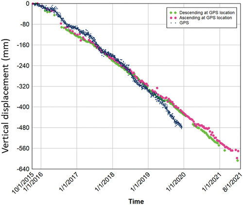
Figure 7. (a) Spatial distribution of the SBAS-InSAR surface vertical deformation result in relation to the main urban landmarks: (b) Narayanhiti Palace, (c) airport, (d) Patan Durbar Square. Building footprints are shown from Microsoft’s GlobalMLBuildingFootprints dataset (https://github.com/microsoft/GlobalMLBuildingFootprints). The four black dots in (a) are the locations of the four deep water wells used in stratigraphic column analysis.
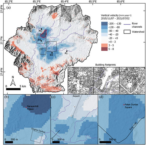
Figure 8. (a) InSAR vertical velocity and sediment thickness crossplot within the entire watershed area. Each dot represents a pixel value of 130 × 130 m in size. There is a basic positive correlation of increased sediment thickness with increasing vertical subsidence velocity around −10 mm year−1. A cluster of high subsidence rate points (<-130 mm year−1) is located near Narayanhiti Palace (the red contour area in Figure 7). (b) The InSAR vertical velocity and DTM crossplot within the entire watershed area. Each dot represents a pixel value of 130 × 130 m. The red vertical line at the zero point differentiates those points uplifting and subsiding.
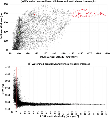
Figure 9. (a) Stratigraphy column from four deep water wells across the basin shows shallow and deep aquifers. This figure illustrates the representative stratigraphic columns of the Kathmandu basin, based on the lithological logs obtained from deep wells. The locations of these wells are indicated on the map (see ). The basin-fill sediments are categorized into three stratigraphic units. The ‘SG’ unit predominantly consists of sand and gravel layers, indicative of paleo-fluvial and early lacustrine deposits. These units, including the top weathering surface of the bedrock (‘BR’), exhibit favourable aquifer characteristics and serve as a significant water source for deep water tube wells in the basin. The ‘Cs’ unit is primarily comprised of clay and silt, interspersed with sandy lenses. It predominantly represents lacustrine sediments that deposited during periods where water ponded in the basin. The thickness of this unit varies from a few metres to approximately 300 metres. The sandy lenses and silt layers within this unit also serve as water sources for water wells in the basin. The top ‘Sa’ represents a mainly sandy sequence deposited after the basin drainage. It serves as a suitable aquifer for shallow wells, receiving recharge during the rainy season (data source: (DMG Citation1988; Pandey et al. Citation2023)). (b) Four deep water well locations have been analysed using InSAR time-series to show their LOS subsidence rates. In Figure 8a, locations of well P1, P2 and D1 show a clear linear correlation between vertical velocity and sediment thickness, while D2 deviates from this trend. Figure 9a illustrates how the ambiguous boundaries of D2’s shallow and deep aquifers in the stratigraphic column might account for this uncertainty.
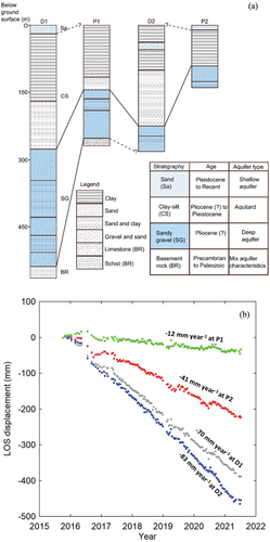
Figure 10. InSAR vertical velocity and DTM crossplot. Each dot represents a pixel size of 130 × 130 m. The red dots show the points that are along the river channel that cover a 130 m area, due to the pixel size. Within a small sample area around the Kathmandu Valley’s central rivers (indicated by the black dotted polygon in Figure 4a), linear trends show increasing vertical velocities with rising elevation. The lower values along the river channels are likely associated with recharging from the river to its immediate surroundings.
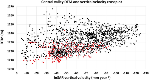
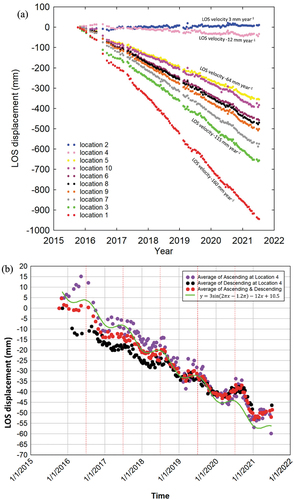
Figure 11. (a) Time-series from the ascending frame at 10 different locations indicated in triangles in Figure 4a. (b) Averaged time-series at location 4 from both the ascending and descending frames. The annual sinusoidal signal is marked by red dotted lines that peak in the month of July. Because the raw result from the SBAS-InSAR is velocity from the line-of-sight direction, the time-series plots the changes of accumulated line-of-sight displacement with time.