
Figures & data
Figure 1. HyperScout-1 pushframe imaging technique.
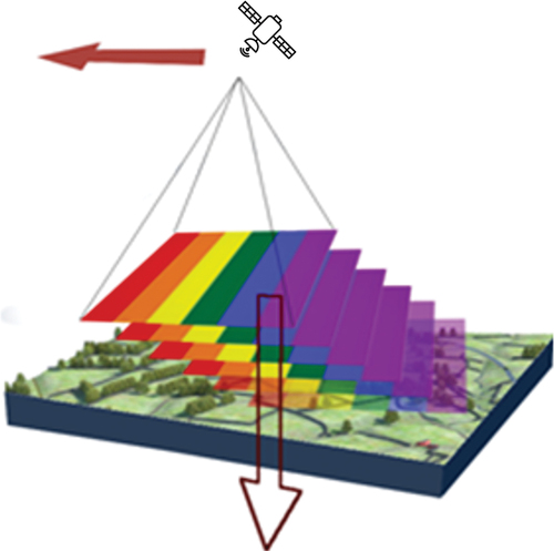
Table 1. HyperScout-1 main characteristics.
Figure 2. HyperScout-1: example spectral responses of a set of 36 adjacent lines. Blue line with circles shows the combined spectral response of a single spectral band.
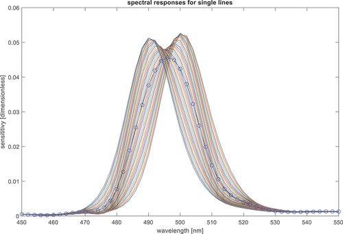
Figure 3. HyperScout-1 instrument spectral band characteristics (top) spectral responses (bottom) full width half max (blue line) and spectral sampling (orange line).
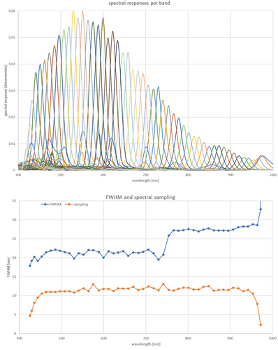
Figure 4. Focal plane layout (a) is the showing the different frame arrangement (sensor, frame, optical and illuminated). (b) is showing the sensor and LVF configuration geometry. The north vector is counter to the satellite motion vector for acquisitions on the descending node, which is the nominal case for out of eclipse acquisitions. The pixel size of the CMV12000 is 5.5 µm whereas the focal plane is 41.25 mm (source: Cosine measurement systems).
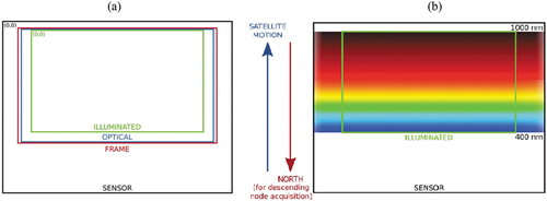
Table 2. HyperScout-1 products description.
Table 3. HyperScout-1 acquisition scenes and their targeted purposes (source: Cosine measurement systems).
Table 4. HyperScout-1 acquired ROIs and their instrument settings. ACT means across track and ALT means along track (source: Cosine measurement systems).
Figure 5. Example of GCPs extracted from GLS2010; left: example of Landsat-7 tile, right: extracted GCPs in 4 spectral bands.
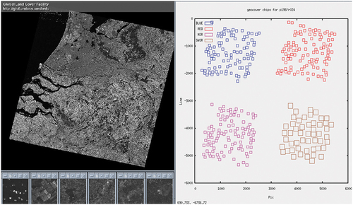
Figure 6. GCP location in the raw data.
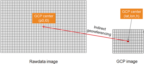
Figure 7. GCPs template searching techniques.
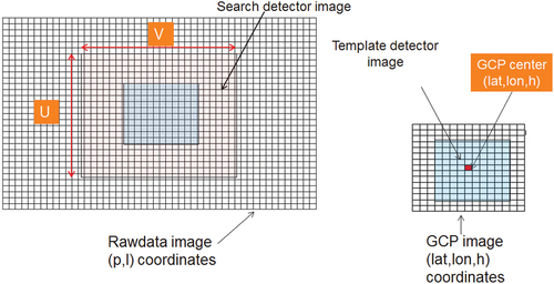
Figure 8. Spectral calibration: modelled and measured spectra with indication of spectral features (spectra scaled for viewing purposes).
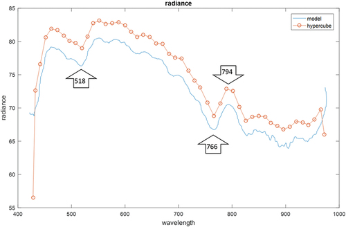
Table 5. HyperScout-1 spectral calibration results.
Figure 9. Radiances for the ‘20181107.01_Libya4’ site: blue) generated using the OSCAR model, orange) with HyperScout-1 spectral responses applied, yellow) HyperScout-1 results with pre-flight calibration.
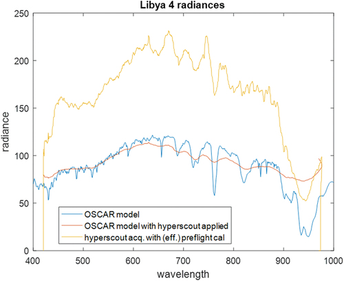
Figure 10. ‘20181107.02_Railroad_Valley’ image, corrected with results of left: band-based calibration, right: line based calibration.
Figure 11. Radiances for Railroad Valley site using sentinel-2 multispectral bands.
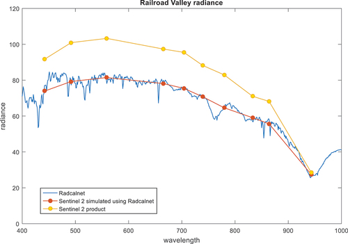
Figure 12. Radiances for the Railroad Valley site using the (corrected) RadCalNet model, and derived from the hyperscout-1 acquisition and inflight calibration parameters.
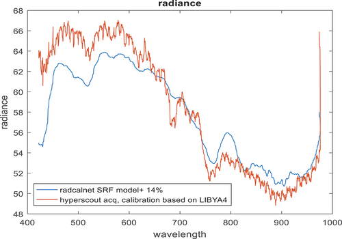
Table 6. Initial absolute geolocation errors for all processed ROIs.
Figure 13. Observed shift between successive frames. The image is a false colour RGB image (R: projected frame#1, G: projected frame#2, and B: projected frame#2).
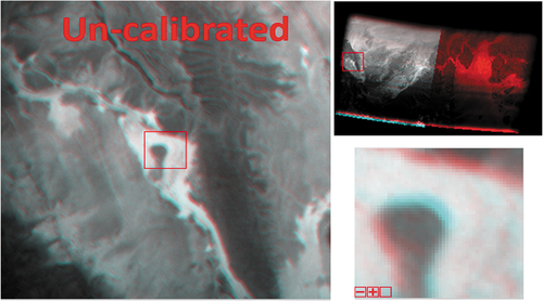
Figure 14. Observed shift between further away frames. The image is a false colour RGB image (R: projected frame#1, G: projected frame#15, and B: projected frame#15).
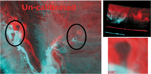
Figure 15. Illustration of the GCP selection performed for the ‘20181108.01_Algeria’ site. The GCPs were extracted from the Landsat global land survey CGP database (see section 5.3.1). The green areas are the Landsat scenes intersecting with the HyperScout-1 ROI bounding box.
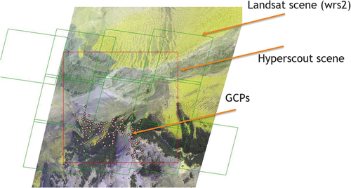
Figure 16. Measured initial focal plane distortion in across track (top) and along track (bottom) direction observed for all frame acquired above the ‘20181108.01_Algeria’ site. Each dot is representing a GCP distortion measurement and each colour is representing a frame (in total 15 frames were processed).
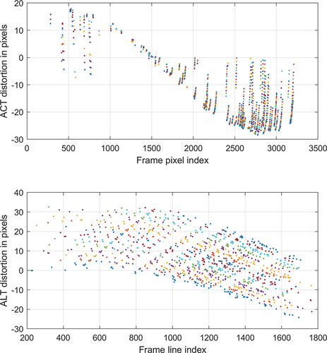
Figure 17. Geometric absolute error (top: across track; bottom: along track). Green points show the error before calibration and the black points show the error after calibration.
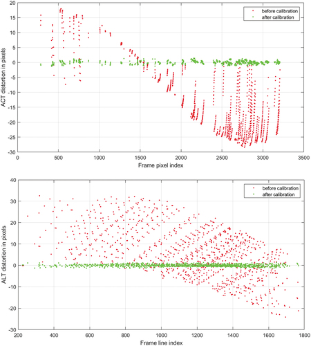
Table 7. Table showing per frame, the geometric error in across and along track (in pixels) before and after the calibration.