Comparative analysis of multispectral data between GF-1 WFV4 and GF-6 WFV sensors

Figures & data

Table 1. GF-1 WFV4 and GF-6 WFV satellite orbit parameters.

parameter	GF-1 WFV4	GF-6 WFV
Orbit type	Sun synchronous orbit	Sun synchronous orbit
Revisitation period/d	4	4
Orbital altitude	645 km	644.5472 km
Orbit inclination	98.0506º	97.9597°
Local time of descending node	10:30 AM	10:30 AM
Return to the circle times	605	605
Return period	41 Day	41 Day

Table 2. GF-1 WFV4 and GF-6 WFV satellite sensor parameters.

Parameter		GF-1 WFV4	GF-6 WFV
Launch time		2013/4/26	2018/6/2
Camera type		Wide field of view camera (WFV)	Wide field of view camera (WFV)
Radiometric resolution/bit		10	12
Spatial resolution/m		16	16
Width/km		200	800
Spectral range/μm	B1	0.45–0.52	0.45–0.52
	B2	0.52–0.59	0.52–0.59
	B3	0.63–0.69	0.63–0.69
	B4	0.77–0.89	0.77–0.89

Figure 1. GF-1 WFV4 (a–c) vs. GF-6 WFV (e–f) image pairs (RGB: 432). (a)–(c) show the GF-1 WFV4 data for the three regions, (d)–(f) show the GF-6 WFV data for the three regions.

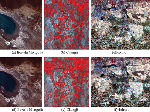
Table 3. The location and size of the image pairs in the study area.

Study area	Latitude	Longitude	pixel numbers
Bortala Mongolia	44°39′59”−45°3′21“N	82°56′38”−83°24′52“E	2659×2272
Changji	43°45’29”−43°57′43“N	89°26′38“−89°42′08” E	1383×1260
Hohhot	40°26′00”−40°35′59“N	110°29′16”−110°44′56“E	1384×1161

Table 4. The parameters of the synchronizing image pairs.

Image pairs	Sensor	date	Time	Solar zenith (°)	Solar azimuth (°)	Satellite zenith (°)	Satellite Azimuth(°)	Roll satellite angle (°)
Bortala Mongolia	GF1-WFV4	2020/11/06	14:00:32	61.15	175.41	35.66	286.75	7.999
	GF6-WFV		13:32:18	61.44	175.09	6.33	25.63	−0.003
Changji	GF1-WFV4	2020/07/25	13:30:12	25.50	155.88	26.60	285.88	0.000
	GF6-WFV		12:56:19	25.15	151.21	12.97	72.06	−8.993
Hohhot	GF1-WFV4	2020/11/09	11:58:02	57.47	171.62	26.59	285.18	0.000
	GF6-WFV		11:29:58	57.47	171.97	12.99	71.85	−9.005

Table 5. The calibration coefficients for GF-1 WFV4 and GF-6 WFV.

Sensor	Band	Gain	Bias
GF1-WFV4	B1	0.2522	0.000
	B2	0.2029	0.000
	B3	0.1528	0.000
	B4	0.1031	0.000
GF6-WFV	B1	0.0675	0.000
	B2	0.0552	0.000
	B3	0.0513	0.000
	B4	0.0314	0.000

Table 6. The solar irradiance at the TOA of GF-1 WFV4 and GF-6 WFV.

Senor	Band	$\mathit{ESU}{N}_{\lambda }$
GF1-WFV4	B1	1968.08
	B2	1841.53
	B3	1540.8
	B4	1069.6
GF6-WFV	B1	1952.16
	B2	1847.43
	B3	1554.76
	B4	1074.06

Figure 2. The plot of the corresponding band sample area against the y=x line in the sample area by the TOA mean method.

Figure 3. The plot of the corresponding band sample area against the y=0 line in the sample area by the TOA mean method.

Figure 4. Scatter plot of corresponding bands based on ROI spectral mean comparison method for two images.

Table 7. The statistical characteristics related to image pairs in the sample area by the TOA mean comparison method.

	Band	GF-1 WFV4				GF-6 WFV				ME	MAPE/%	R^2	RMSE
		Min	Max	Range	Mean	Min	Max	Range	Mean
Bortala Mongolia	Blue	0.166	0.464	0.298	0.282	0.134	0.379	0.245	0.258	0.024	9.45	0.9892	0.0267
	Green	0.127	0.472	0.345	0.270	0.100	0.445	0.345	0.240	0.030	12.53	0.9848	0.0325
	Red	0.091	0.470	0.379	0.253	0.089	0.459	0.370	0.239	0.014	5.75	0.9815	0.0200
	NIR	0.057	0.479	0.422	0.248	0.065	0.448	0.383	0.234	0.013	5.76	0.9799	0.0229
Changji	Blue	0.085	0.280	0.195	0.127	0.102	0.197	0.095	0.146	−0.018	12.65	0.978	0.0193
	Green	0.076	0.314	0.238	0.134	0.084	0.287	0.203	0.142	−0.008	5.51	0.9739	0.0116
	Red	0.051	0.310	0.259	0.132	0.067	0.307	0.240	0.146	−0.014	9.80	0.9866	0.0167
	NIR	0.051	0.430	0.379	0.243	0.072	0.411	0.339	0.256	−0.013	4.94	0.9872	0.0195

Figure 5. Scatter plot of the corresponding band in the sample area by the TOA mean comparison method in Hohhot.

Table 8. The statistical characteristics before and after the simulation of apparent reflectivity in Hohhot.

Band	MAPE				RMSE
	Blue	Green	Red	NIR	Blue	Green	Red	NIR
Before simulation	−2.1615	2.9379	−2.6882	−1.9331	0.0127	0.0201	0.0219	0.0218
After simulation	−1.1862	−0.7441	−0.7028	−0.3076	0.0109	0.0177	0.0201	0.0205
Variation (%)	−0.98	−2.19	−1.99	−1.63	−14.11	−12.23	−8.46	−6.08

Figure 6. The scatter versus the y=0 line for the corresponding band in the sample area of Hohhot.

Figure 7. Typical features extraction diagram. (a)–(g) Binarization images of water bodies in Bortala Mongolia, where (a) is the NDWI validation data; (b) is the water body binarization map of the GF-6 WFV image with a threshold of 0.14; (c) is the water body binarization map of the GF-1 WFV4 image with a threshold of 0.14; (d) is the water body binarization map of the GF-1 trans WFV image with a threshold of 0.14; (e) is the water body binarization map of the GF-6 WFV image with a threshold of 0.20. (f) is the water body binarization map of the GF-1 WFV4 image with a threshold of 0.20, (g) is the water body binarization map of the GF-1 trans WFV image with a threshold of 0.20.(h)–(n) the vegetation binarization images of the Changji area, where (h) is the NDVI validation data; (i) is the vegetation binarization map of the GF-6 WFV image with a threshold of 0.42; (j) is the vegetation binarization map of the GF-1 WFV4 image with a threshold of 0.42; (k) is the vegetation binarization map of the GF-1 trans WFV image with a threshold of 0.42; (l) is the vegetation binarization maps of the GF-6 WFV image with a threshold of 0.46, (m) is the vegetation binarization maps of the GF-1 WFV4 image with a threshold of 0.46, (n) is the vegetation binarization maps of the GF-1 trans WFV image with a threshold of 0.46.

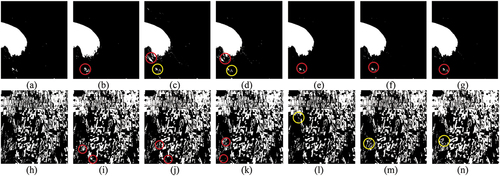
Table 9. Typical feature extraction thresholds and Kappa coefficient statistics.

Region	Sensor	Threshold	Kappa1	Threshold	Kappa 2	Validate the data
Bortala Mongolia NDWI	GF-1 WFV4	0.14	0.9470	0.20	0.9614	Landsat8
	GF-6 WFV	0.14	0.9615	0.20	0.9522	Landsat8
	GF-1 trans WFV	0.14	0.9528	0.20	0.9603	Landsat8
Changji NDVI	GF-1 WFV4	0.42	0.9193	0.46	0.9285	Landsat8
	GF-6 WFV	0.42	0.9222	0.46	0.9074	Landsat8
	GF-1 trans WFV	0.42	0.9204	0.46	0.9291	Landsat8

During the feature extraction process, combining the index method with threshold adjustment effectively enhances visualization and ensures good consistency with validation data (as shown in Figure 7). It is noteworthy that the data transformed from GF-6 to GF-1 trans are closer to the original GF-1 data in vegetation and water body extraction, rather than GF-6. Even when the threshold is set to 0.42 or 0.46, the visual differences between GF-1 and GF-6 in surface cover feature extraction are not significant.

Figure 8. The plot of water bodies ROI in the corresponding bands in Bortala Mongolia and Hohhot versus y=0.

Figure 9. The plot of the vegetation ROI in the corresponding bands in Changji and Hohhot versus.

Figure 10. Relative Spectral Response of GF-1 WFV4 and GF-6 WFV.

Data availability statement

The data that support the findings of this study are available from the corresponding author, upon reasonable request.