Evaluating the Suitability of Multi-Scale Terrain Attribute Calculation Approaches for Seabed Mapping Applications

Figures & data

Table 1. Five multi-scale approaches for calculating terrain attributes (Dolan and Lucieer 2014). Asterisks denote marine examples.

#	Method	Abbreviated name	Published examples
1	Resample DTM then calculate attribute	Resample-calculate	Rengstorf et al. (2012)*, Gottschalk et al. (2011)
2	Average DTM then calculate attribute	Average-calculate	Giusti, Innocenti, and Canese (2014)*
3	Calculate attribute then average	Calculate-average	Misiuk, Lecours, and Bell (2018)*
4	Calculate attribute using variable k × k window	k × k-window	Bargain et al. (2017)*, Porskamp et al. 2018)*, Trzcinska et al. (2020)*
5	Multiple integrated spatial scales	Integrated-multiscale	Gorini and Mota (2011), Lindsay and Newman (2018), Lecours and Espriella (2020)*, Shang et al. (2021)*

Figure 1. Locations of study sites at (A) D’Argent Bay, Newfoundland and Labrador, Canada, and (B) the Bjørnøya slide and surrounding area on the Norwegian continental margin. Source: Author, country borders were obtained from the ESRI Countries WGS84 layer.

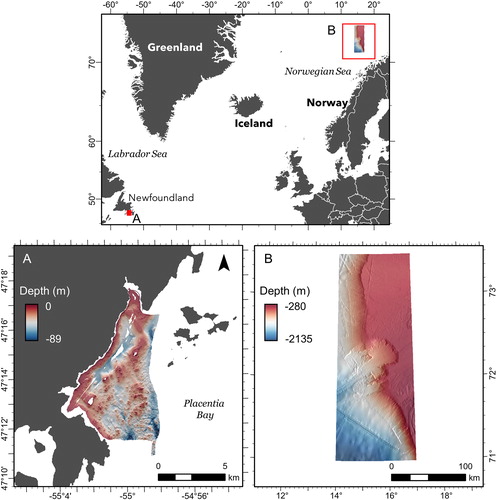
Figure 2. Calculating raster terrain attributes at analysis distance D_t = 45 m using four different multi-scale methods: (A) ‘resample-calculate’, (B) ‘average-calculate’, (C) ‘calculate-average’, and (D) ‘k × k-window’. Parameters at the bottom of each pane describe the aggregation window size (j), focal window size (k), cell length (l_c), cell neighborhood size (m_c), and attribute calculation distance (D_i). Solid borders represent the focal cell; bold borders represent D_i. Note that for (B) and (C), the analysis distance (D_t) of calculations at the focal cell is extended to 45 m by the aggregation windows of each neighboring cell within the 3 × 3 focal window.

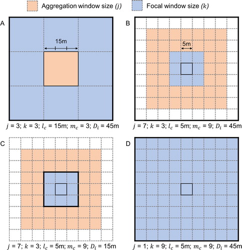
Table 2. Example of scale manipulation parameters over ten analysis distances (D_t) based on multi-scale calculation method, applied to a 5 m resolution input dataset. An example with a 250 m resolution input dataset is provided in the Appendix. Note how D_i and D_t vary relative to the other parameters and each other.

Resample bathymetry, calculate attribute (‘resample-calculate’)
Agg. window size j (cells)	1	3	5	7	9	11	13	15	17	19
Focal window size k (cells)	3	3	3	3	3	3	3	3	3	3
Cell length lc (m)	5	15	25	35	45	55	65	75	85	95
Cell neighborhood size mc (cells)	3	3	3	3	3	3	3	3	3	3
Attr. calculation distance Di (m)	15	45	75	105	135	165	195	225	255	285
Analysis distance Dt (m)	15	45	75	105	135	165	195	225	255	285
Average bathymetry, calculate attribute (‘average-calculate’)
Agg. window size j (cells)	1	3	5	7	9	11	13	15	17	19
Focal window size k (cells)	3	3	3	3	3	3	3	3	3	3
Cell length lc (m)	5	5	5	5	5	5	5	5	5	5
Cell neighborhood size mc (cells)	3	5	7	9	11	13	15	17	19	21
Attr. calculation distance Di (m)	15	25	35	45	55	65	75	85	95	105
Analysis distance Dt (m)	15	25	35	45	55	65	75	85	95	105
Calculate attribute, average attribute (‘calculate-average’)
Agg. window size j (cells)	1	3	5	7	9	11	13	15	17	19
Focal window size k (cells)	3	3	3	3	3	3	3	3	3	3
Cell length lc (m)	5	5	5	5	5	5	5	5	5	5
Cell neighborhood size mc (cells)	3	5	7	9	11	13	15	17	19	21
Attr. calculation distance Di (m)	15	15	15	15	15	15	15	15	15	15
Analysis distance Dt (m)	15	25	35	45	55	65	75	85	95	105
Calculate attribute over k × k window (‘k × k-window’)
Agg. window size j (cells)	1	1	1	1	1	1	1	1	1	1
Focal window size k (cells)	3	5	7	9	11	13	15	17	19	21
Cell length lc (m)	5	5	5	5	5	5	5	5	5	5
Cell neighborhood size mc (cells)	3	5	7	9	11	13	15	17	19	21
Attr. calculation distance Di (m)	15	25	35	45	55	65	75	85	95	105
Analysis distance Dt (m)	15	25	35	45	55	65	75	85	95	105

Figure 3. Hillshaded 5 m resolution bathymetry at D’Argent Bay. A terrain profile from West to East (A) shows topographic features at several scales. Finer-scale features are superimposed on broader ones (B).

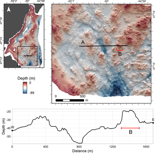
Figure 4. Relative difference to the mean value (RDMV) at the transect in Figure 3A across ten analysis distances (D_t) using four different multi-scale calculation methods at D’Argent Bay. Values at the finest scale (red) describe correspondingly small topographic features; values at moderate (green) and broad (purple) scales differ substantially between methods. Dashed lines indicate the extent of the feature indicated in Figure 3B.

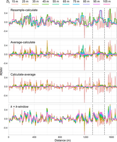
Figure 5. Slope at the transect in Figure 3 calculated across ten analysis distances (D_t) using four different multi-scale calculation methods at D’Argent Bay. Slope details and flat areas are averaged out using the ‘calculate-average’ method. Dashed lines indicate the extent of the feature indicated in Figure 3B.

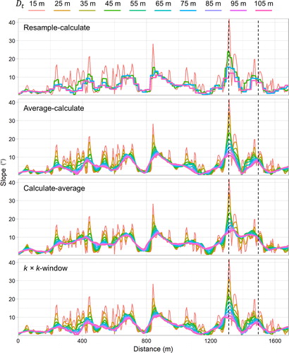
Figure 6. Hillshaded slope at D’Argent Bay. The magnified area shows features along the terrain profile. At analysis distance D_t = 15 m (A), an arrow indicates the feature discussed in the text and annotated in Figure 3. The scale of the slope layers is increased to D_t = 65 m using (B) ‘calculate-average’ and (C) ‘k × k-window’ methods. The color ramp is clipped to a maximum of 20° to facilitate comparison between maps.

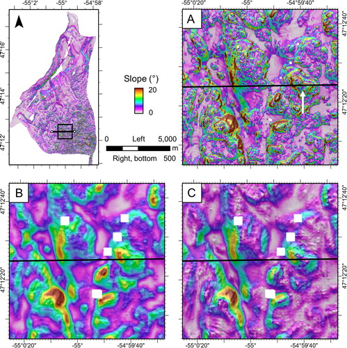
Figure 7. Average correlation and entropy statistics of terrain attributes compared to the finest scale using each multi-scale calculation method at D’Argent Bay. Error bars show the standard deviations of all variables at each analysis distance.

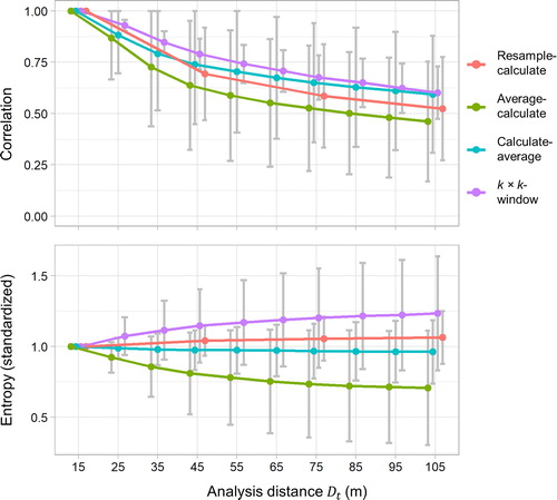
Figure 8. Hillshaded 250 m resolution GEBCO bathymetry (left) and data source identified via type identifier (TID) grid (right) at the Bjørnøya slide. A terrain profile from North to South (A; bottom) crosses what appears to be a dataset compilation boundary (at B) near the crown of the slide. Note that the pre-generated grid sections contain multiple data sources and are not necessarily of uniform quality/resolution. The pre-generated grid data south of B comprise full-coverage multibeam bathymetry from which more consistent terrain attributes are expected.

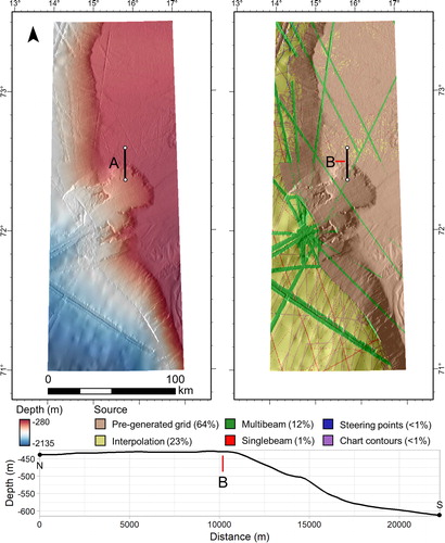
Figure 9. Effects of terrain attribute calculation methods on multisource data compilation (A) artefacts at the Bjørnøya slide. Relative difference to the mean value (RDMV) and eastness at analysis distance D_t = 750 m (B, G) are increased to D_t = 3,750 using ‘resample-calculate’ (C, H), ‘average-calculate’ (D, I), ‘calculate-average’ (E, J), and ‘k × k-window’ (F, K) methods. The data compilation boundary identified in Figure 8 is indicated by the dashed red line in (A).

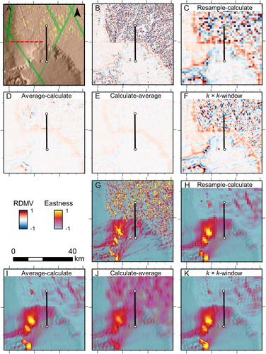
Figure 10. Eastness from North to South (left to right) at the profile in Figures 8 and 9 calculated across ten analysis distances (D_t) using four different multi-scale calculation methods at the Bjørnøya slide. Vertical dashed lines show approximate locations of the slide crown (black) and dataset compilation boundary (red).

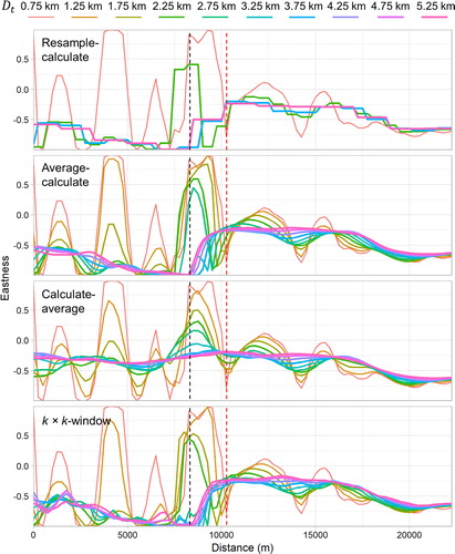
Figure 11. Scaled (0-1) absolute error between all terrain attribute values at ‘actual’ and ‘measured’ sample sites for multiple analysis distances at D’Argent Bay. Box plots show the error distributions at analysis distances that can be achieved using all multi-scale calculation methods (i.e., including ‘resample-calculate’), with means at all scales displayed as circles.

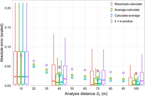
Table 3. Comparison of relative suitability of multi-scale calculation methods for the three purposes identified in this study.

Purpose	Criteria	Multi-scale method performance				Comments
		Resample- calculate	Average- calculate	Calculate- average	k × k- window
Characterize specific features or processes.	Maximize new and unique information at the target scale.	Good	Poor	Poor	Good	‘k × k’ and ‘resample-calculate’ methods were effective. Selection depends on the desired resolution.
Reduce data compilation artefacts.	Minimize influence of artefacts on the terrain attribute.	Mixed	Mixed	Mixed	Poor	‘Average-calculate’ reduced the magnitude of artefacts, but also reduced terrain information.
Match positional accuracy of ground-truth.	Minimize error between terrain attribute values at ‘measured’ and ‘actual’ sample locations.	Poor	Good	Good	Poor	‘Calculate-average’ provided the greatest reduction in sample locational error.

Table A1. Example of scale manipulation parameters over ten analysis distances (D_t) based on multi-scale calculation method, applied to a 250 m resolution input dataset.

Resample bathymetry, calculate attribute (‘resample-calculate’)
Agg. window size j (cells)	1	3	5	7	9	11	13	15	17	19
Focal window size k (cells)	3	3	3	3	3	3	3	3	3	3
Cell length lc (m)	250	750	1250	1750	2250	2750	3250	3750	4250	4750
Cell neighborhood size mc (cells)	3	3	3	3	3	3	3	3	3	3
Attr. calculation distance Di (m)	750	2250	3750	5250	6750	8250	9750	11250	12750	14250
Analysis distance Dt (m)	750	2250	3750	5250	6750	8250	9750	11250	12750	14250
Average bathymetry, calculate attribute (‘average-calculate’)
Agg. window size j (cells)	1	3	5	7	9	11	13	15	17	19
Focal window size k (cells)	3	3	3	3	3	3	3	3	3	3
Cell length lc (m)	250	250	250	250	250	250	250	250	250	250
Cell neighborhood size mc (cells)	3	5	7	9	11	13	15	17	19	21
Attr. calculation distance Di (m)	750	1250	1750	2250	2750	3250	3750	4250	4750	5250
Analysis distance Dt (m)	750	1250	1750	2250	2750	3250	3750	4250	4750	5250
Calculate attribute, average attribute (‘calculate-average’)
Agg. window size j (cells)	1	3	5	7	9	11	13	15	17	19
Focal window size k (cells)	3	3	3	3	3	3	3	3	3	3
Cell length lc (m)	250	250	250	250	250	250	250	250	250	250
Cell neighborhood size mc (cells)	3	5	7	9	11	13	15	17	19	21
Attr. calculation distance Di (m)	750	750	750	750	750	750	750	750	750	750
Analysis distance Dt (m)	750	1250	1750	2250	2750	3250	3750	4250	4750	5250
Calculate attribute over k × k window (‘k × k-window’)
Agg. window size j (cells)	1	1	1	1	1	1	1	1	1	1
Focal window size k (cells)	3	5	7	9	11	13	15	17	19	21
Cell length lc (m)	250	250	250	250	250	250	250	250	250	250
Cell neighborhood size mc (cells)	3	5	7	9	11	13	15	17	19	21
Attr. calculation distance Di (m)	750	1250	1750	2250	2750	3250	3750	4250	4750	5250
Analysis distance Dt (m)	750	1250	1750	2250	2750	3250	3750	4250	4750	5250

Figure A1. Average correlation and entropy statistics of terrain attributes compared to the finest scale using each multi-scale calculation method at the Bjørnøya slide. Standard deviations are shown by the error bars.

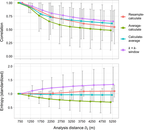
Figure A2. Eastness at D’Argent Bay at analysis distance D_t = 15 m (A) is increased to D_t = 65 m using (B) ‘resample-calculate’, (C) ‘average-calculate’, (D) ‘calculate-average’, and (E) ‘k × k-window’ methods.

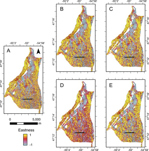
Figure A3. Relative difference to the mean value (RDMV) at D’Argent Bay at analysis distance D_t = 15 m (A) is increased to D_t = 65 m using (B) ‘resample-calculate’, (C) ‘average-calculate’, (D) ‘calculate-average’, and (E) ‘k × k-window’ methods.

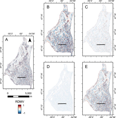
Figure A4. Bathymetric standard deviation at D’Argent Bay at analysis distance D_t = 15 m (A) is increased to D_t = 65 m using (B) ‘resample-calculate’, (C) ‘average-calculate’, (D) ‘calculate-average’, and (E) ‘k × k-window’ methods.

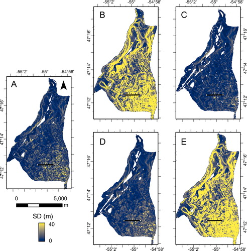
Figure A5. Slope at D’Argent Bay at analysis distance D_t = 15 m (A) is increased to D_t = 65 m using (B) ‘resample-calculate’, (C) ‘average-calculate’, (D) ‘calculate-average’, and (E) ‘k × k-window’ methods.

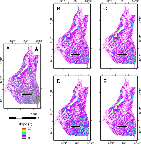
Figure A6. Vector ruggedness measure (VRM) at D’Argent Bay at analysis distance D_t = 15 m (A) is increased to D_t = 65 m using (B) ‘resample-calculate’, (C) ‘average-calculate’, (D) ‘calculate-average’, and (E) ‘k × k-window’ methods.

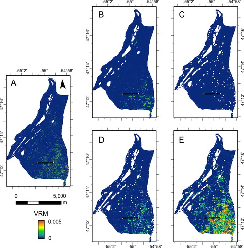
Figure A7. Eastness at the transect in Figure 3 calculated across 10 analysis distances (D_t) using four different multi-scale methods at D’Argent Bay.

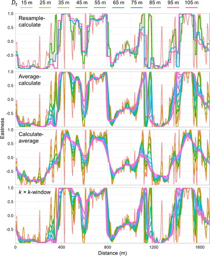
Figure A8. Bathymetric standard deviation at the transect in Figure 3 calculated across 10 analysis distances (D_t) using four different multi-scale methods at D’Argent Bay.

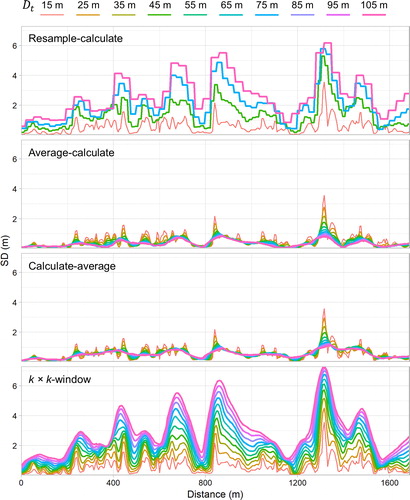
Figure A9. Vector ruggedness measure (VRM) at the transect in Figure 3 calculated across 10 analysis distances (D_t) using four different multi-scale methods at D’Argent Bay.

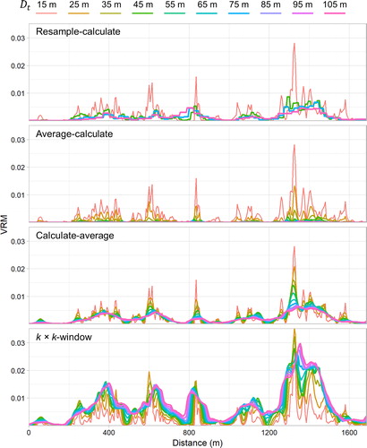
Figure A10. Eastness at the Bjørnøya slide at analysis distance D_t = 750 m (A) is increased to D_t = 3,750 m using (B) ‘resample-calculate’, (C) ‘average-calculate’, (D) ‘calculate-average’, and (E) ‘k × k-window’ methods.

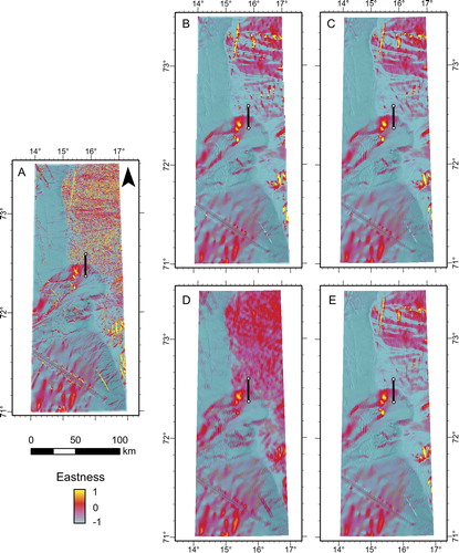
Figure A11. Relative difference to the mean value (RDMV) at the Bjørnøya slide at analysis distance D_t = 750 m (A) is increased to D_t = 3,750 m using (B) ‘resample-calculate’, (C) ‘average-calculate’, (D) ‘calculate-average’, and (E) ‘k × k-window’ methods.

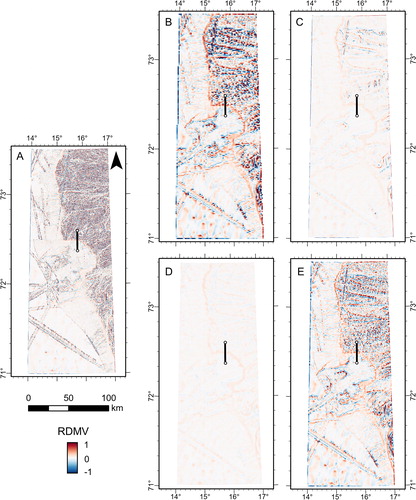
Figure A12. Bathymetric standard deviation at the Bjørnøya slide at analysis distance D_t = 750 m (A) is increased to D_t = 3,750 m using (B) ‘resample-calculate’, (C) ‘average-calculate’, (D) ‘calculate-average’, and (E) ‘k × k-window’ methods.

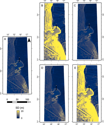
Figure A13. Slope at the Bjørnøya slide at analysis distance D_t = 750 m (A) is increased to D_t = 3,750 m using (B) ‘resample-calculate’, (C) ‘average-calculate’, (D) ‘calculate-average’, and (E) ‘k × k-window’ methods.

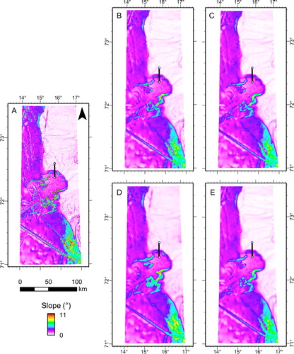
Figure A14. Vector ruggedness measure (VRM) at the Bjørnøya slide at analysis distance D_t = 750 m (A) is increased to D_t = 3,750 m using (B) ‘resample-calculate’, (C) ‘average-calculate’, (D) ‘calculate-average’, and (E) ‘k × k-window’ methods.

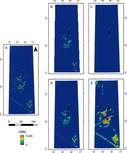
Figure A15. Relative difference to the mean value (RDMV) from North to South (left to right) at the profile in Figure 8 calculated across 10 analysis distances (D_t) using four different multi-scale methods at the Bjørnøya slide. Vertical dashed lines show approximate locations of the slide crown (black) and dataset compilation boundary (red).

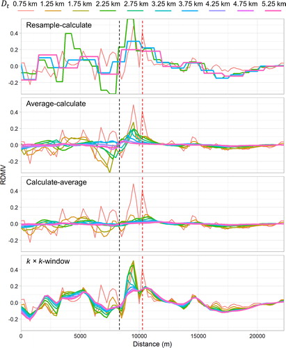
Figure A16. Bathymetric standard deviation from North to South (left to right) at the profile in Figure 8 calculated across 10 analysis distances (D_t) using four different multi-scale methods at the Bjørnøya slide. Vertical dashed lines show approximate locations of the slide crown (black) and dataset compilation boundary (red).

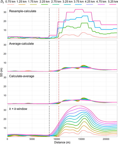
Figure A17. Slope from North to South (left to right) at the profile in Figure 8 calculated across 10 analysis distances (D_t) using four different multi-scale methods at the Bjørnøya slide. Vertical dashed lines show approximate locations of the slide crown (black) and dataset compilation boundary (red).

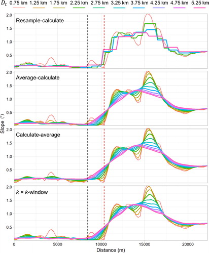
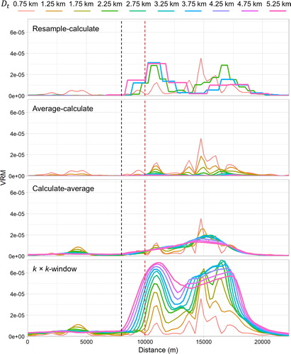
Figure A18. Vector ruggedness measure (VRM) from North to South (left to right) at the profile in Figure 8 calculated across 10 analysis distances (D_t) using four different multi-scale methods at the Bjørnøya slide. Vertical dashed lines show approximate locations of the slide crown (black) and dataset compilation boundary (red).

Dolan, M. F. J., and V. L. Lucieer. 2014. Variation and uncertainty in bathymetric slope calculations using geographic information systems. Marine Geodesy 37 (2):187–219.

 Web of Science ®Google Scholar

Rengstorf, A. M., A. Grehan, C. Yesson, and C. Brown. 2012. Towards high-resolution habitat suitability modeling of vulnerable marine ecosystems in the deep-sea: Resolving terrain attribute dependencies. Marine Geodesy 35 (4):343–61.

 Web of Science ®Google Scholar

Gottschalk, T. K., B. Aue, S. Hotes, and K. Ekschmitt. 2011. Influence of grain size on species–habitat models. Ecological Modelling 222 (18):3403–12.

 Web of Science ®Google Scholar

Giusti, M., C. Innocenti, and S. Canese. 2014. Predicting suitable habitat for the gold coral Savalia savaglia (Bertoloni, 1819) (Cnidaria, Zoantharia) in the South Tyrrhenian Sea. Continental Shelf Research 81:19–28.

 Web of Science ®Google Scholar

Misiuk, B., V. Lecours, and T. Bell. 2018. A multiscale approach to mapping seabed sediments. PLoS ONE 13 (2):e0193647.

 PubMed Web of Science ®Google Scholar

Bargain, A., F. Marchese, A. Savini, M. Taviani, and M.-C. Fabri. 2017. Santa Maria di Leuca Province (Mediterranean Sea): Identification of suitable mounds for cold-water coral settlement using geomorphometric proxies and Maxent methods. Frontiers in Marine Science 4:338.

 Web of Science ®Google Scholar

Porskamp, P., A. Rattray, M. Young, and D. Ierodiaconou. 2018. Multiscale and hierarchical classification for benthic habitat mapping. Geosciences 8 (4):119.

 Web of Science ®Google Scholar

Trzcinska, K., L. Janowski, J. Nowak, M. Rucinska-Zjadacz, A. Kruss, J. S. von Deimling, P. Pocwiardowski, and J. Tegowski. 2020. Spectral features of dual-frequency multibeam echosounder data for benthic habitat mapping. Marine Geology 427:106239.

 Web of Science ®Google Scholar

Gorini, M. A. V., and G. L. A. Mota. 2011. Which is the best scale? Finding fundamental features and scales in DEMs. In Proceedings of Geomorphometry 2011, 67–70. Redlands, CA.

 Google Scholar

Lindsay, J. B., and D. R. Newman. 2018. Hyper-scale analysis of surface roughness. Preprint. PeerJ Preprints. https://peerj.com/preprints/27110v1.

 Google Scholar

Shang, X., K. Robert, B. Misiuk, J. Mackin-McLaughlin, and J. Zhao. 2021. Self-adaptive analysis scale determination for terrain features in seafloor substrate classification. Estuarine, Coastal and Shelf Science 254:107359.

 Web of Science ®Google Scholar

Data availability statement

The GEBCO_2019 bathymetry data supporting the findings in this study are available for free from the GEBCO data portal: https://www.gebco.net/data_and_products/gridded_bathymetry_data/gebco_2019/gebco_2019_info.html. Access to the D’Argent Bay multibeam data will be considered upon request by the authors.