
Figures & data
Figure 1. Zodiac boat used as GNSS-based sea level measurement system since 2012. GNSS receiver is on-board and connected to the antenna located at the rear.
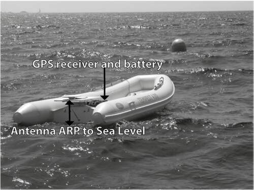
Figure 2. Photos of CalNaGeo. Left: for offshore use (open ocean; two inflatable boats) during this experiment (the GNSS-Zodiac can be seen on the right in the background and the lighthouse, where the reference receiver is, on the left in the background). Right: for inshore use (coastal ocean, lakes, rivers; one inflatable boat) during a campaign on the Seine river, France in June 2017. Middle: zoom on the gimbal system (photo from another experiment).
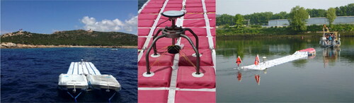
Figure 3. Left: Full experiment area (orange rectangle corresponds to the zoom at right). Right: Zoom on the area where tide gauges are located. Purple and Red lines are the Jason and Sentinel-3A ground tracks respectively. Colored contour map and black lines from GPS measurements during the 1999 Catamaran experiment (Bonnefond et al. Citation2003). White lines from CalNaGeo GPS measurements during the 2015 experiment (this study). Red dots for tide gauges (M3 and M5 in this study). Yellow circles mark the 250 m distance to compare SSH from GNSS and tide gauges. The GNSS-Zodiac was anchored at about 90 m Westward from the M5 tide gauge (blue anchor on the Figure). Grey cross for the permanent GNSS receiver (G0 in the lighthouse area, upper left in right hand panel).
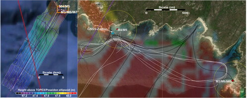
Figure 4. SSH differences with M5 tide gauge when within 250 m (cngh – M5) as a function of time without corrections (green crosses, ), with geoid corrections (red crosses, see Table S5 under the Section “Additional tables and figures” in the supplemetary file) and with both geoid and weighted and smoothed crossovers corrections (cyan crosses, ): top, middle and bottom for “Short”, “Air” and “iPPP” GPS solutions respectively. Dashed vertical black lines correspond to Eastward passes close to M5. Solid vertical black lines correspond to Westward passes close to M5. Orange vertical lines correspond to beginning and end of the phases when cngh was static (close to M5 and zodi, see –5). The horizontal dashed lines correspond to the mean for static periods (orange, inside vertical orange lines) and periods with velocity (grey, outside vertical orange lines) for the solutions with both geoid and weighted and smoothed crossovers corrections (cyan crosses).
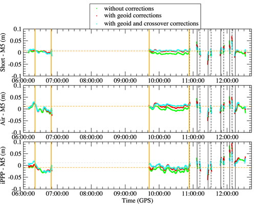
Figure 5. Top: SSH tidal signal (height above the TOPEX/Poseidon ellipsoid) for M3 tide gauge (black line), M5 tide gauge (red line) and average of M3 and M5 tide gauges (green line). Bottom: SSH differences between M3 and M5 tide gauges.
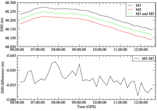
Figure 6. Examples of crossovers: raw GNSS positions at 1 Hz (orange line and crosses), raw SSH crossovers (cyan crosses) and averaged SSH crossovers from raw ones (purple diamonds, annotated values correspond to the averaged time difference). Left: One track crosses another one (main horizontal and vertical ticks every ∼10 m). Right: One track follows another one (main horizontal and vertical ticks every ∼100 m).
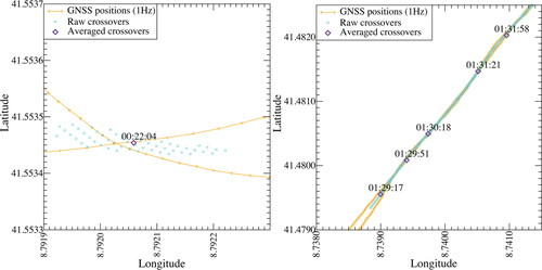
Figure 7. SSH differences at crossovers as a function of time (top left) and as a function of time differences (top right), for “Short” (black crosses), “Air” (red diamonds) and “iPPP” (green circles) GNSS solutions. Bottom: histogram of the time differences (time lag) at crossovers.
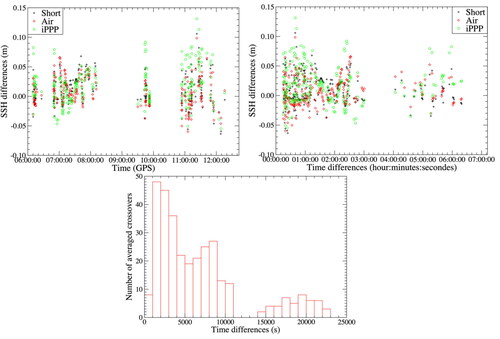
Table 1. SSH crossover differences for different processing strategies and tide corrections.
Figure 8. Averaged crossover corrections as a function of time (blue crosses), linearly interpolated at 1 Hz solution time (red dots), with a weighted (normalized time difference) moving average (width = 300 s/Step = 30 s, orange dots) and finally smoothed by a 60 s low-pass filter (green dots). Time differences are given in annotated values. Top: period with high density of crossovers. Right: period with low density of crossovers.
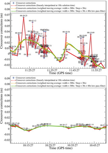
Figure 9 SSH differences for zodi (top) and cngh (bottom): “Air - Short” (black lines), “iPPP - Short” (red lines) and “iPPP - Air” (green lines) G solutions respectively. Horizontal lines correspond to the mean of each set of differences (see ).
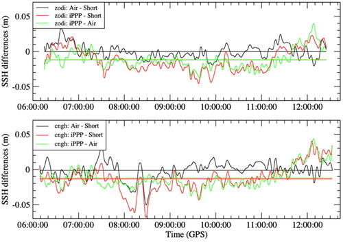
Table 2. SSH differences statistics without any outliers’ removal for the different processing strategies and type of instruments and for all epochs (1 Hz).
Table 3. Statistics of SSH differences with M5 tide gauge (zodi – M5) within 250 m (velocity < 0.3 m/s). Values in brackets correspond to common data in time with cngh (see ).
Table 4. Statistics of SSH differences with M5 tide gauge (cngh – M5) within 250 m (velocity < 0.3 m/s). Values in brackets correspond to common data in time with zodi (see ).
Table 5. Statistics of SSH differences with M5 tide gauge (cngh – M5) within 250 m (velocity < 0.3 m/s) with weighted and smoothed (see Section “Crossover correction”) crossover corrections (using M3&M5 tide correction, see ) and with geoid corrections (see also Table S4 under the Section “Additional tables and figures” in under the supplemetary file). Values in brackets (separated by a “/”) are for the first and second period of static measurements respectively (see vertical orange lines in ).
Table 6. Statistics of SSH differences with M5 tide gauge (cngh – M5) within 250 m (for all velocities). Values in brackets correspond to common data in time with the ones with geoid correction (see in this section and Table S5 under the Section “Additional tables and figures” in the supplemetary file).
Table 7. Statistics of SSH differences with M5 tide gauge (cngh – M5) within 250 m (for all velocities) with weighted and smoothed (see Section “Crossover correction”) crossover corrections (using M3&M5 tide correction, see ) and with geoid corrections.
Table 8. Linear trend of SSH differences with M5 tide gauge (cngh – M5) within 250 m as a function of velocity (from 0.3 to 6 m/s). Values in brackets from a linear regression based on a “robust” least absolute deviation method (ladfit.pro IDL routine). “±” is the formal error from the regression process.
Figure 10. SSH differences with M5 tide gauge (cngh – M5) within 250 m as a function of velocity (from 0.3 to 6 m/s) without corrections (green crosses), with geoid corrections (red crosses) and with both geoid and weighted and smoothed crossovers corrections (cyan crosses) (corresponding color lines for the linear regressions, see values in ): top, middle and bottom for “Short”, “Air” and “iPPP” GNSS solutions respectively. Black dash curves correspond to a quadratic fit for the “geoid and weighted and smoothed crossovers corrections” sets.
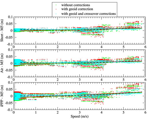
Figure 11. SSH differences with M5 tide gauge (cngh – M5) as a function of the distance to the coast (M5) without (black lines) or with (red lines) weighted and smoothed crossovers corrections (both corrected from geoid): top, middle and bottom for “Short”, “Air” and “iPPP” GNSS solutions respectively. Solid red lines and dashed black ones are for the linear regression for the remaining slope shown in (note that being very close, the dashed black line is masked by the solid red one). Statistics (mean, standard deviation…) are given in .
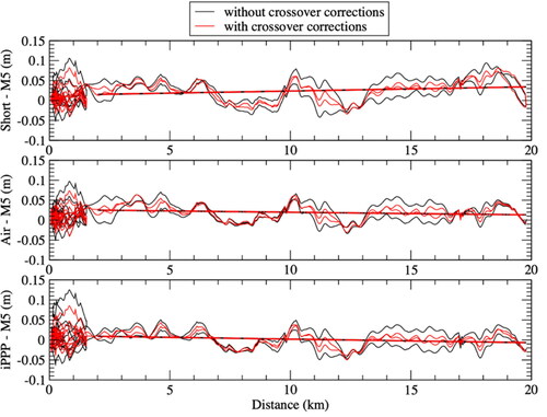
Table 9. Linear trend of SSH differences (cngh – M5) as a function distance to the coast (from 2 to 20 km). The poor agreement between 0 and 2 km has been excluded because it corresponds to the area where the stability of CalNaGeo waterline was tested and is not in the same along-track direction. “±” is the formal error from the regression process.
Supplemental Material
Download MS Word (4.6 MB)Data availability statement
The data that support the findings of this study are available from the corresponding author [PB], upon reasonable request.