Using infinite server queues with partial information for occupancy prediction

Figures & data

Figure 1. Phases of the prison system.

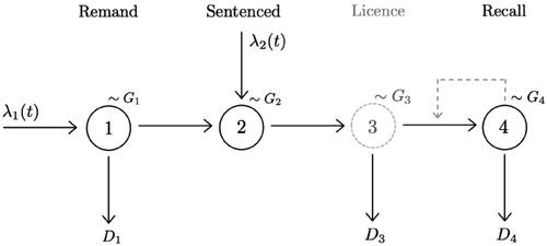
Figure 2. Regions describing arrival and service pairs (u, v).

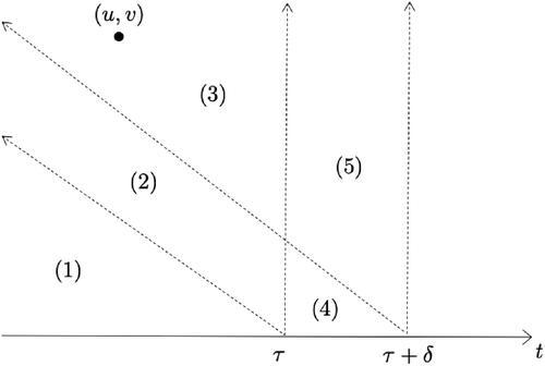
Figure 3. Left to right: density plots of marginal posterior distributions for parameters β₀, β₁, α and θ.

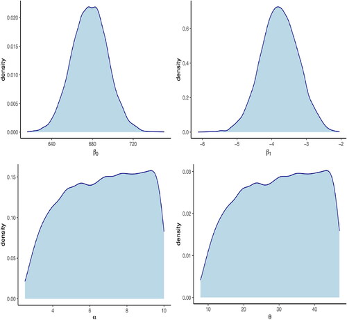
Figure 4. Prediction of the number of prisoners in the Theft offences group from August 2019 to March 2020. Left panel: long-term projections (red line) together with two standard deviation prediction interval (grey shaded region). Right panel: short-term projections (red line) together with two standard deviation prediction interval (grey shaded region). The observed values are in black.

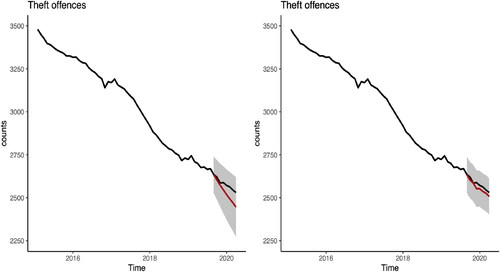
Figure 5. Prediction of the number of prisoners in the Sexual offences (top row) and Public order offences (bottom row) groups from August 2019 to March 2020. Left panel: long-term projections (red line) together with two standard deviation prediction interval (grey shaded region). Right panel: short-term projections (red line) together with two standard deviation prediction interval (grey shaded region). The observed values are in black.

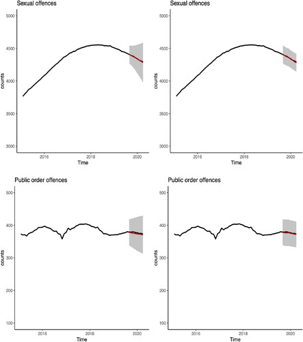
Figure 6. Example 4.3. Sentencing policy modification for Theft offences group where $E[S^o]=5.22.$ The red line is associated with unchanged parameters, the blue line is associated with $E[S^{\nu }]=8$ and the green line with $E[S^{\nu }]=3.$ Solid line is the predictor. Dashed lines represent two standard deviation prediction intervals.

Figure 7. Example 4.3. Sentencing policy modification for Sexual offences group where $E[S^o]=29.71.$ The red line is associated with unchanged parameters, the blue line is associated with $E[S^{\nu }]=48$ and the green line with $E[S^{\nu }]=24.$ Solid line is the predictor. Dashed lines represent two standard deviation prediction intervals.

Figure 8. Example 4.3. Sentencing policy modification for Public order offences group where $E[S^o]=3.79.$ The red line is associated with unchanged parameters, the blue line is associated with $E[S^{\nu }]=12$ and the green line with $E[S^{\nu }]=1.$ Solid line is the predictor. Dashed lines represent two standard deviation prediction intervals.

Figure 9. Example 3.7. For fixed $E[S]=3,$ varying $(\lambda ,c_s^2).$

Figure C11. ARIMA model prediction of the number of prisoners in the Theft offences group from August 2019 to March 2020. Left panel: long-term projections (red line) together with two standard deviation prediction interval (grey shaded region). Right panel: short-term projections (red line) together with two standard deviation prediction interval (grey shaded region). The observed values are in black.

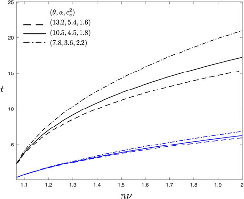
Figure C10. Example B.2. Congestion level relative to the mean $n\nu$ vs. recovery time $t.$ For fixed $E[S]=3,$ $\nu =30$ and varying $(\theta ,\alpha ,c_s^2)$ (black lines). An intervention of ${\lambda }_2=0.8{\lambda }_1$ is illustrated by the corresponding blue lines.

Figure C12. ARIMA model prediction of the number of prisoners in the Sexual offences (top row) and Public order offences (bottom row) groups from August 2019 to March 2020. Left panel: long-term projections (red line) together with two standard deviation prediction interval (grey shaded region). Right panel: short-term projections (red line) together with two standard deviation prediction interval (grey shaded region). The observed values are in black.

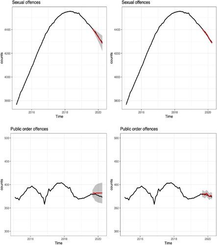
Table 1. Offence groups.

1.	Violence against the person	7.	Possession of weapons
2.	Sexual offences	8.	Public order offences
3.	Robbery	9.	Miscellaneous crimes against society
4.	Theft Offences	10.	Fraud Offences
5.	Criminal damage and arson	11.	Summary Non-Motoring
6.	Drug offences	12.	Summary motoring