Adaptive Multivariate Global Testing

Figures & data

Table 1. Model and prior parameters of the z* and t*-tests, respectively, and their dimension

Parameters	Dimension	Parameters	Dimension
	(K^2 + 5K)/2		K^2 + 3K
	2K
	2		3K

Figure 1. Power (left panel) and (right panel) versus sample allocation ratio. We plot the sequential χ²-test (magenta ) and the z* (green − − line), sequential z (cyan −), and z⁺ (orange − ·) tests with first stage/fixed/first step weighting vector 0 (×), 30° (), 60° () and 90° () angle to the optimal. The remaining design parameters are J = 2, K = 10, α = 0.05, α_{1, 1} = 0.01, α_{0, 1} = 1, n_T = 60, n₀ = 0.5n₁, .

Figure 2. Power of the t*-test versus Mahalanobis distance for various . In the left panel, the vectors while in the right panel and which, for (green − × − line), give and 72°, respectively. In both panels, are also chosen to give ϕ = 25° (dark green − ○ − line), 45° (dark green − + − line) and 65° (dark green − ⋄ − line). The remaining design parameters are J = 2, K = 10, α = 0.05, α_{1, 1} = 0.01, α_{0, 1} = 1, n_T = 20, r = 0.5, n₀ = 0.75n₁, ν₀ = n₀ − 1.

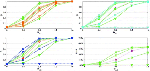
Figure 3. Power and versus Mahalanobis distance. We plot the z*-test (green − −) with the tests z⁺ (orange − .) (up left), sequential z (cyan −) and χ² (magenta · ⋄ ·) (up right), single stage z (blue −) and χ² (red · ⋄ ·) (down left) and sequential χ² (down right). The linear combination z*/z/z⁺ tests are performed with first stage/fixed/first step weighting vectors having 0 (×), 30° (), 60° (), and 90° () angle to the optimal. The remaining design parameters are J = 2, K = 10, α = 0.05, α_{1, 1} = 0.01, α_{0, 1} = 1, n_T = 30, r = 0.5, n₀ = 0.75n₁, ν₀ = n₀ − 1.

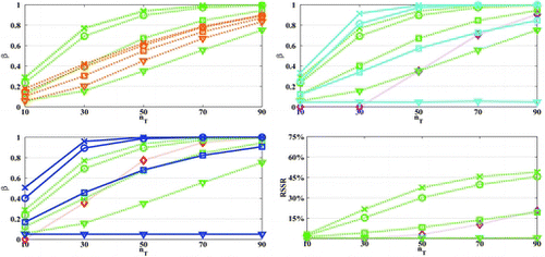
Figure 4. Power and versus the total sample size n_T. We plot the t*-test (green − −) with the tests, t⁺ (orange − .) (up left), sequential t (cyan −) and T² (magenta · ⋄ ·) (up right), single stage t (blue −) and T² (red · ⋄ ·) (down left) and sequential T² (down right). The linear combination t*/t/t⁺ tests are performed with first stage/fixed/first step weighting vectors having 0 (×), 30° (), 60° (), and 90° () angle to the optimal. The remaining design parameters are K = 15, J = 2, α = 0.05, α_{1, 1} = 0.01, α_{0, 1} = 1, r = 0.5, n₀ = 6, ν₀ = n₀ − 1, .

Table 2. Means, standard deviations, correlations, and their prior estimates for the EEG depression study presented in Läuter, Glimm, and Kropf (1996)

ch.	3	4	5	6	7	8	17	18	19
	0.8710	1.5890	1.0370	1.1460	0.8510	0.8530	1.4220	0.7510	0.9950
m0, k	0.5	3.50	1	2	2	2	2	2	2
	2.9494	3.5121	2.3637	2.2490	2.2760	2.0706	3.2624	2.6382	2.3593
s0, k	1.5	2.5	1	2	2	2	2	2	2
	1	0.9262	0.8115	0.7959	0.5786	0.4902	0.9323	0.4896	0.5312
4	0.8	1	0.6270	0.7835	0.3357	0.4450	0.9313	0.2778	0.4892
5	0.8	0.7	1	0.7882	0.8492	0.7173	0.7347	0.7145	0.7611
6	0.7	0.8	0.7	1	0.6020	0.7924	0.8180	0.6334	0.7783
7	0.5	0.4	0.7	0.55	1	0.6155	0.4639	0.6833	0.5992
8	0.4	0.5	0.55	0.7	0.6	1	0.5177	0.5983	0.7833
17	0.9	0.9	0.75	0.75	0.45	0.45	1	0.4048	0.5711
18	0.45	0.45	0.65	0.65	0.7	0.7	0.5	1	0.4445
19	0.75	0.75	0.8	0.8	0.65	0.65	0.8	0.7	1

Läuter, J., Glimm, E., Kropf, S. (1996), New Multivariate Tests for Data With an Inherent Structure, Biometrical Journal, 38, 1–23.

 Google Scholar