2,977
Views
23
CrossRef citations to date
0
Altmetric
Applications and Case Studies

Unifying Amplitude and Phase Analysis: A Compositional Data Approach to Functional Multivariate Mixed-Effects Modeling of Mandarin Chinese

Pages 545-559 | Received 01 Jun 2015, Published online: 06 Jul 2015

Figures & data

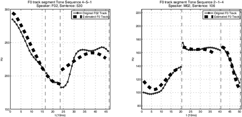
Figure 1 An example of triplet trajectories from speakers F02 and M02 over natural time. F(emale)02 tonal sequence: 4-5-1, M(ale)02 tonal sequence: 2-1-4; Mandarin Chinese rhyme sequences [oŋ-@-iou] and [ien-in-], respectively. See supplementary material for full contextual covariate information.

Table 1 Covariates examined in relation to F0 production in Taiwanese Mandarin. Tone variables in a 5-point scale representing tonal characterization, 5 indicating a toneless syllable, with 0 representing the fact that no rhyme precedes the current one (such as at the sentence start). Reference tone trajectories are shown in the supplementary material section: Linguistic Covariate Information

Figure 2 Summary of the overall estimation procedure resulting in the estimates of the functional principal components and scores via the covariates in the linear mixed effect model.
Figure 3 The multivariate mixed effects model presented exhibits a crossed (nonbalanced) random structure. The vowel-rhyme curves (V) examined are cross-classified by their linguistic (Sentence—Pi) and their nonlinguistic characterization (Speaker—Si).
Figure 4 Corresponding amplitude variation functions w (top row) and phase variation functions h (bottom row) functions for the triples shown in .
Figure 4 Corresponding amplitude variation functions w (top row) and phase variation functions h (bottom row) functions for the triples shown in Figure 1.
Figure 5 Functional estimates (continuous curves) are shown superimposed of the corresponding original discretized speaker data over the physical time domain t.
Figure 6 W (amplitude) eigenfunctions Φ: mean function ([0.05, 0.95] percentiles shown in gray) and first, second, third, fourth, fifth, and sixth functional principal components (FPCs) of amplitude.

Table 2 Percentage of variances reflected from each respective FPC (first 9 shown). Cumulative variance in parenthesis

Table 3 Actual deviations in Hz from each respective FPC (first 9 shown). Cumulative deviance in parenthesis. (Human speech auditory sensitivity threshold ≈ 10 Hz)

Figure 7 (Phase) eigenfunctions Ψ: mean function ([0.05, 0.95] percentiles shown in gray) and first, second, third, fourth, fifth, and sixth functional principal components (FPCs) of phase. Roughness is due to differentiation and finite grid; the corresponding warping functions in their original domain are given in Figure S.1 in the supplementary material.

Table 4 Random effects std. deviations
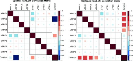
Figure 8 Random effects correlation matrices. The estimated correlation between the variables of the original multivariate model (Equation Equation(3.19)) is calculated by rescaling the variance-covariance submatrices ΣR1 and ΣR22 of ΣΓ to unit variances. Each cell i, j shows the correlation between the variance of component in row i that of column j; row/columns 1–4: wFPC1-4, row/columns 5–8: sFPC1-4, row/columns 9: Duration.
Figure 8 Random effects correlation matrices. The estimated correlation between the variables of the original multivariate model (Equation Equation(3.19)An×p=XN×kBk×p+ZN×lΓl×p+EN×p,) is calculated by rescaling the variance-covariance submatrices ΣR1 and ΣR22 of ΣΓ to unit variances. Each cell i, j shows the correlation between the variance of component in row i that of column j; row/columns 1–4: wFPC1-4, row/columns 5–8: sFPC1-4, row/columns 9: Duration.
Supplemental material

Supplementary Materials

Download Zip (247.8 KB)