Meta-Analysis of Mid-p-Values: Some New Results based on the Convex Order

Figures & data

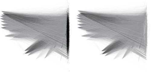
Figure 1. Authentication data: Full network of connections comprising $\sim 18\text{,}000$ nodes and $\sim 400\text{,}000$ directed edges. Edges are colored by authentication type. On the left, nodes are shown as black points, with node ID “C17693” highlighted in red (and larger). On the right, the points are hidden to better see the connections made by node ID “C17693,” which are now highlighted in pink.

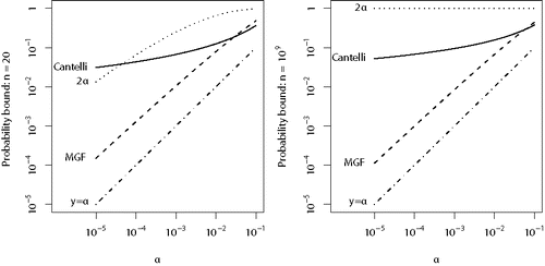
Figure 2. Comparison of the probability bounds given by Theorem 2 for Fisher’s method using mid-p-values. Theorem 2 gives explicit formulas for 2α, Cantelli and MGF, in that order. Both axes are on the logarithmic scale.

Figure 3. Fisher’s method with discrete p-values. Empirical distribution functions of Fisher’s combined p-value under different conditions. 50/50: Each p-value is equal to 1/2 or 1 (with probability 1/2 each under ${\tilde{H}}_0$). Random binary: Each p-value is equal to p or 1 (with probability p and 1 − p, respectively, under ${\tilde{H}}_0$). p is drawn uniformly on [0, 1] (independently of whether ${\tilde{H}}_0$ or ${\tilde{H}}_1$ holds). Grid of 10: Each p-value is drawn from 1/10, 2/10…, 1 (with probability 1/10 each under ${\tilde{H}}_0$). n = 10, β = 20: 10 p-values from a left-censored Beta(1, 20) distribution. n = 100, β = 5: 100 p-values from a left-censored Beta(1, 5) distribution. Dotted line: Randomized p-values. Solid line: Mid-p-value. Dashed line: Standard p-values. Further details in the main text.