Nonparametric Estimation of Copula Regression Models With Discrete Outcomes

Figures & data

Fig. 1 $H_1(s;X_1)$ (solid curve) as a function of $\mu =X_1^{\prime }{\beta }_1$ for Poisson GLM with the log link. Dashed curves: $F_1(k|X_1)$, from left to right $k=0,1,2,3,4,5,15$, and 16. The curve of $H_1(s;X_1)$ is composed of pieces from the curves of $F_1(k|X_1),k=0,\dots$. Horizontal lines: $s+ϵ,s$, and $s-ϵ$.

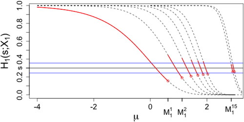
Fig. 2 $H_1(s;X_1)$ (solid curve) as a function of $\mu =X_1^{\prime }{\beta }_1$ for logistic regression (left panel) and ordinal regression with 4 levels (right panel). Dashed curves for right panel: $F_1(k|X_1)$, from left to right k = 0, 1, 2. Horizontal lines: $s+ϵ,s,s-ϵ$.

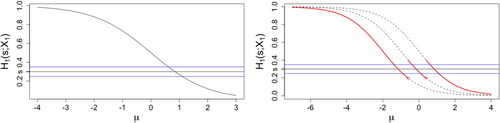
Fig. 3 Contour plots of the nonparametric estimator for Poisson outcomes under different scenarios with sample size 1000. The average of the estimator over 500 replications is given by the solid lines, while the dash-dot symbols give the corresponding $95\%$ confidence interval for every other copula value, and the dashed lines give the underlying copulas.

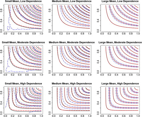
Fig. 4 Contour plots of $f_{H(s,t;\mathbf{X})}(s,t)$ for Poisson outcomes under different marginal mean levels.

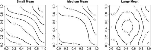
Fig. 5 Contour plots of the nonparametric estimator for Poisson outcomes under different scenarios with sample size 5000.

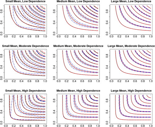
Table 1 ISE values for Poisson examples under different scenarios (multiplied by 1000).

		n = 1000		n = 5000
Marginal mean	Dependence	Average	SD	Average	SD
Small	Low	2.865	2.081	0.857	0.311
	Moderate	3.061	2.233	0.878	0.334
	High	3.547	2.652	0.974	0.429
Medium	Low	0.331	0.118	0.107	0.030
	Moderate	0.330	0.125	0.101	0.030
	High	0.352	0.150	0.103	0.031
Large	Low	0.088	0.040	0.018	0.009
	Moderate	0.088	0.040	0.018	0.009
	High	0.091	0.047	0.019	0.010

Fig. 6 Left panel: contour plot of $f_{H(s,t;\mathbf{X})}(s,t)$ for binary outcomes. Right panel: contour plot of the nonparametric estimator for binary outcomes with sample size 5000.

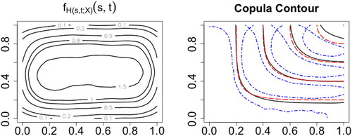
Fig. 7 Contour plots of the empirical copula estimator (solid curve) with its confidence interval (dash-dot symbols) compared with the underlying copulas (dashed lines).

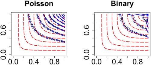
Table 2 ISE of three-dimensional estimator for Poisson outcomes under high dependence with sample size 5000 (multiplied by 1000).

Marginal Mean	Average	SD
Small	2.500	1.408
Medium	0.143	0.042
Large	0.017	0.008

Table 3 Empirical numbers of observations.

	Total	0	1	2	3	4	5	>5
BC	5660	3976	997	333	136	76	31	111
MV	2175	1511	314	116	53	36	21	124
Joint	2170

Table 4 Description and summary statistics of covariates.

Variable	Description	Mean
TypeCity	=1 if entity type is city	0.140
TypeCounty	=1 if entity type is county	0.058
TypeSchool	=1 if entity type is school	0.282
TypeTown	=1 if entity type is town	0.173
TypeVillage	=1 if entity type is village	0.237
TypeMisc	=1 if entity type is other	0.110
NoClaimCreditBC	=1 if no building and content claims
	in prior year given BC coverage	0.328
NoClaimCreditMV	=1 if no MV claims
	in prior year given MV coverage	0.054
lnCoverageBC	Coverage of BC line in logarithmic	2.119
	millions of dollars given BC coverage	(2.000)
lnCoverageMV	Coverage of MV line in logarithmic	−0.798
	millions of dollars given MV coverage	(1.626)
lnDeductBC	BC deductible level in logarithmic	7.155
	millions of dollars given BC coverage	(1.174)

Table 5 Correlations between frequencies of claims.

Kendall’s τ	Spearman’s ρ
0.361	0.402

Table 6 Marginal coefficients.

		BC (0-1 inflated Poisson)		MV (Negative Binomial)
	Variable Name	Coef.	SE	Coef.	SE
Count	(Intercept)	−1.540	0.125	−0.929	0.109
	lnCoverage	0.751	0.023	0.708	0.036
	lnDeduct	−0.020	0.017
	NoClaimCredit	−0.395	0.131	−0.370	0.146
	TypeCity	−0.143	0.079	0.231	0.149
	TypeCounty	−0.250	0.087	1.518	0.132
	TypeMisc	−0.195	0.179	−0.352	0.301
	TypeSchool	−1.157	0.085	0.651	0.131
	TypeTown	0.186	0.175	−1.085	0.244
	size			1.428	0.139
Zero	(Intercept)	−4.755	0.448
	lnCoverage	−0.580	0.078
	lnDeduct	0.879	0.062
	NoClaimCredit	0.536	0.280
One	(Intercept)	−5.533	0.639
	lnCoverage	−0.047	0.094
	lnDeduct	0.577	0.084
	NoClaimCredit	0.300	0.353

Fig. 8 Contour plot of the nonparametric estimator (solid) and its confidence intervals (dotted) compared with parametric copulas contours (dashed).

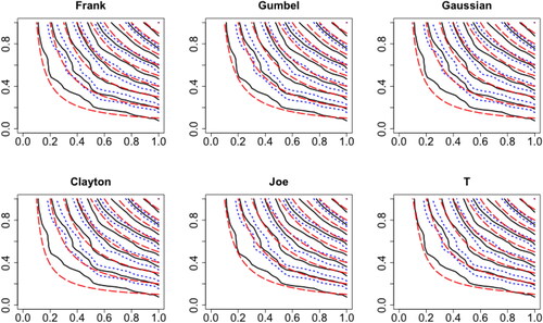
Table 7 Parameters from different parametric copulas.

	Estimate	SE	Kendall’s τ
Gumbel	1.040	0.015	0.038
Joe	1.042	0.018	0.024
T(df = 4)	0.072	0.038	0.046
Frank	0.718	0.221	0.079
Gaussian	0.125	0.033	0.079
Clayton	0.223	0.075	0.100

Table 8 Distances $d(\widehat{C}(·;\widehat{\beta }),{\tilde{C}}_{\widehat{\theta }})$ of different parametric copulas (multiplied by 1000).

	Gumbel	Joe	t	Frank	Gaussian	Clayton
Estimate	0.633	0.635	0.646	0.711	0.701	0.885
SE	0.240	0.251	0.240	0.239	0.237	0.265

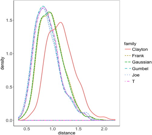
Fig. 9 Density plot of the distances (multiplied by 1000) of different parametric copulas.