Detecting Abrupt Changes in the Presence of Local Fluctuations and Autocorrelated Noise

Figures & data

Fig. 1 Segmentations of well-log data: wild binary segmentation using the strengthened Schwarz information criteria (top); segmentation under square error loss with penalty inflated to account for autocorrelation in measurement error (middle); optimal segmentation from DeCAFS with default penalty (bottom). Each plot shows the data (black line) the estimated mean (red line) and changepoint location (vertical blue dashed lines).

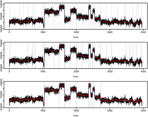
Fig. 2 Top row: projections of data v for detecting a change in the middle of n = 100 data-points. Random walk model (top-left) for varying ${\sigma }_{\eta }^2$ of 0.03 (black), 0.02 (red) and 0.01 (green); AR(1) plus random walk model (top-right) for ${\sigma }_{\eta }^2=0.01$ and varying $\varphi$ of 0.4 (black), 0.2 (red) and 0.1 (green). In both plots the blue line shows the standard cusum projection. Bottom row: noncentrality parameter for a ${\chi }_1^2$ test of a change using the optimal projection (solid line) and the cusum projection (dashed line) for a change of size 1 in the middle of the data as we vary n. Out-fill asymptotics (bottom-left) where $({\sigma }_{\eta }^2,\varphi )$ is (0.0025,0) (black), (0.01,0) (red), (0.0025,0.5) (green) and (0.01,0.5) (blue); In-fill asymptotics (bottom-right) where for n = 50 $({\sigma }_{\eta }^2,\varphi )$ is (0.0025,0) (black), (0.01,0) (red), (0.0025,0.5) (green) and (0.01,0.5) (blue).

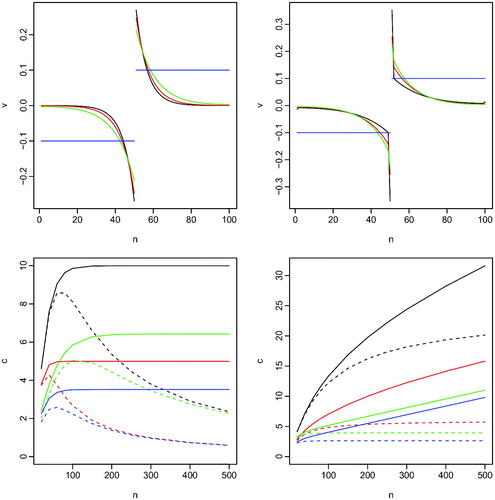
Fig. 3 Four different change scenarios. Top-left, no change present, top-right, change pattern with 19 different changes, bottom-left up changes only, bottom-right, up-down changes of the same magnitude. In this particular example data were generated from an AR model with $\varphi =0.7,{\sigma }_{\nu }=2$.

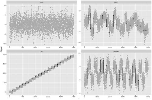
Fig. 4 F1 Scores on the 4 different scenarios. In A a pure AR(1) over a range of values of $\varphi$, for fixed values of ${\sigma }_{\nu }=2,{\sigma }_{\eta }=0$ and a change of magnitude 10. In B a pure AR(1) process with fixed $\varphi =0.85$ and changes in the signal of various magnitudes. In C the full model with $\varphi =0.85$ for a range of values of ${\sigma }_{\eta }$. The gray line represents the cross-section between parameters values in A, B, and C. AR1Seg est. and DeCAFS est. refer to the segmentation of the relative algorithms with estimated parameters. Note, in B the results from DeCAFS and DeCAFS est overlap so only one line is visible. Other algorithms use the true parameter values.

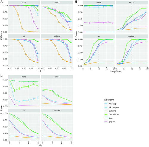
Fig. 5 F1 score on different scenarios with AR(2) noise as we vary ${\varphi }_2$. Data simulated fixing ${\sigma }_{\nu }=2,{\sigma }_{\eta }=0$ and ${\varphi }_1=0.3$ over a change of size 20.

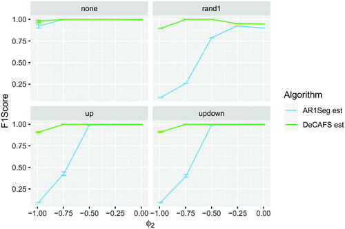
Fig. 6 In A the F1Score on the 4 scenarios for the Sinusoidal Model for fixed amplitude of 15, changes of size 5 and IID Gaussian noise with a variance of 4, as we vary the frequency of the sinusoidal process. In B an example of a realization for the updown scenario, vertical segments refer to estimated changepoint locations of DeCAFS (in light green) and AR1Seg (in blue).

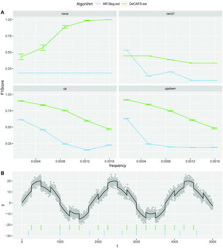
Fig. 7 On top: comparison of the F1 Score in A1, Precision in A2 and MSE in A3, for DeCAFS (in green) and LAVA (in red) with oracle initial parameters and the relative results with estimated initial parameters (in lighter colours), on the updown scenario for a random walk signal over a range of values of ${\sigma }_{\eta }$. On the bottom the first 250 observations of two realizations of the experiment with, in B1, ${\sigma }_{\eta }$ equal to 0.5 and in B2 ${\sigma }_{\eta }$ equal to 2. Again, the continuous lines over the data points represent the signal estimates of DeCAFS and LAVA; and the vertical lines below show their estimated changepoint locations.

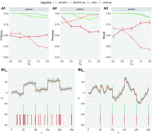
Fig. 8 Data on 2000 bp of the plus-strand of the Bacilus subtilis chromosome. Gray dots show the original data. The plain red line represents the estimated signal of DeCAFS with a penalty of $10\hspace{0.17em}\text{log}\hspace{0.17em}(n)$. The dashed black line represents the estimated signal of hmmTiling.

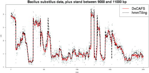
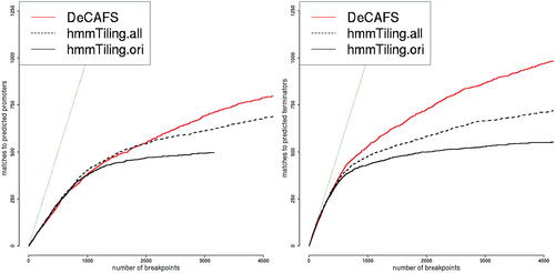
Fig. 9 Benchmark comparisons. The number of promoters (left) and terminators (right) correctly predicted on the plus strand, $M(\delta )$ using a 22 bp distance cutoff, as a function of the number of predicted breakpoints, $R(\delta )$. Plain black lines are the results of hmmTiling (as reported in Figure 4 of Nicolas et al. 2009)). Dotted black lines are the results of hmmTiling when considering all probes rather than only those called transitions. Plain red lines are the results of DeCAFS using $\beta =8\hspace{0.17em}\text{log}\hspace{0.17em}(n)$ for promoters and $5\hspace{0.17em}\text{log}\hspace{0.17em}(n)$ for terminators. These values were learned on the minus strand using a data-driven approach. The thin dark-green leaning line represent $y=x.$

Nicolas, P., Leduc, A., Robin, S., Rasmussen, S., Jarmer, H., and Bessières, P. (2009), “Transcriptional Landscape Estimation From Tiling Array Data Using a Model of Signal Shift and Drift,” Bioinformatics, 25, 2341–2347. DOI: 10.1093/bioinformatics/btp395.

 PubMed Web of Science ®Google Scholar