Reversible Jump PDMP Samplers for Variable Selection

Figures & data

Fig. 1 Sample paths of PDMPs implementing variable selection in one dimension. The left and centre plots show the trajectories for a continuous spike-and-slab prior $0.5\mathcal{N}(0,{\tau }^2)+0.5\mathcal{N}(0,{\tau }^2{c}^2)$ where ${\tau }^2=16$. As c decreases the spike component in the mixture approaches a Dirac mass. The figure on the right is the limiting process where we set the velocity to zero allowing the variable to stay fixed at zero.

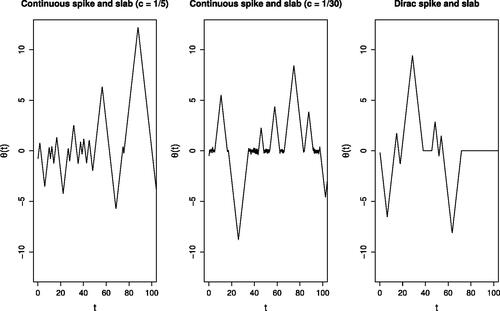
Table 1 Scenario 1 (pair of correlated variables): Relative efficiencies for methods, against a Reversible Jump algorithm, for the marginal posterior means (Mean) and marginal posterior probabilities of inclusion (PI).

	ZigZag		BPS		Gibbs		RJ-HMC
n, d	PI	Mean	PI	Mean	PI	Mean	PI	Mean
100, 100	0.85	4. 83	0.45	4.82	3. 75	4.18	0.03	0.64
200, 100	1.60	33. 98	0.99	24.55	8. 23	8.62	1.35	2.08
400, 100	2.51	47. 03	1.53	35.96	9. 80	9.59	1.58	2.03
800, 100	4.03	39. 94	2.99	33.88	10. 34	11.37	1.43	1.73
100, 200	0.95	0.95	1.32	1.64	4. 54	4. 07	1.25	1.83
200, 200	5.15	42. 90	2.72	28.99	12. 11	11.66	2.01	2.17
400, 200	9.89	76. 29	6.02	48.53	14. 89	13.84	2.20	2.56
800, 200	19.09	160. 99	14.63	91.61	19. 29	19.98	2.39	3.60
100, 400	0.94	1.37	1.66	2.48	3. 38	3. 85	0.44	1.70
200, 400	16.98	80. 38	12.82	55.78	17. 68	16.66	3.17	3.90
400, 400	47. 38	146. 80	29.62	98.08	22.85	22.50	3.88	4.98
800, 400	96. 10	195. 33	50.05	119.00	21.85	21.09	4.03	4.80

NOTE: Bold figures show the best performing sampler.

Table 2 Scenario 2 (General correlation): Relative efficiency for methods, against a Reversible Jump algorithm, for the marginal posterior means (Mean) and marginal posterior probabilities of inclusion (PI). Bold figures show the best performing sampler.

	ZigZag		BPS		Gibbs		RJ-HMC
n, d	PI	Mean	PI	Mean	PI	Mean	PI	Mean
100, 100	0.34	0.67	0.26	1. 21	1. 03	0.82	0.00	0.09
200, 100	0.84	1.27	0.51	1. 86	2. 00	1.22	0.60	0.23
400, 100	1.50	1.98	1.06	2. 62	2. 46	1.80	1.28	1.02
800, 100	2.96	5.38	1.95	5. 60	2. 97	2.46	1.33	1.86
100, 200	0.64	1.05	0.85	1.76	1. 60	1. 95	0.02	1.35
200, 200	1.41	1.49	1.55	2. 43	2. 26	1.16	0.62	0.37
400, 200	3. 84	4.57	3.17	5. 20	3.40	2.38	1.86	2.29
800, 200	6. 45	9. 33	4.16	9.32	4.15	3.67	1.79	2.67
100, 400	1.27	1.50	1.77	2. 44	2. 37	1.75	0.11	1.63
200, 400	3.62	3.65	4.30	6. 04	4. 42	2.95	0.19	1.17
400, 400	14. 96	23.49	13.39	27. 14	8.59	7.59	3.76	5.78
800, 400	23. 48	36. 49	17.44	32.16	8.96	8.47	3.73	5.77

Table 3 Scenario 3 (No correlation): Relative efficiency for methods, against a Reversible Jump algorithm, for the marginal posterior means (Mean) and marginal posterior probabilities of inclusion (PI).

	ZigZag		BPS		Gibbs		RJ-HMC
n, d	PI	Mean	PI	Mean	PI	Mean	PI	Mean
100, 100	0.42	0.87	0.27	1. 53	1. 13	1.06	0.01	0.09
200, 100	0.97	1.34	0.58	2. 03	2. 10	1.47	0.63	0.23
400, 100	1.49	2.03	0.99	2. 25	2. 45	1.62	1.28	0.70
800, 100	2.84	4. 46	1.93	4.37	3. 15	2.23	1.45	1.75
100, 200	0.66	0.70	0.88	1. 58	1. 70	1.57	0.29	0.21
200, 200	1.68	1.44	1.51	1. 89	2. 44	1.49	1.35	0.78
400, 200	5. 37	9.81	4.19	13. 26	4.65	3.42	2.00	2.81
800, 200	8. 69	14.49	6.50	16. 11	5.05	3.83	2.05	2.69
100, 400	0.98	1.37	1.65	2. 50	1. 91	1.55	0.05	1.68
200, 400	2.21	1.94	2.89	2. 89	3. 35	2.20	1.84	2.04
400, 400	6. 98	7.67	6.76	10. 45	5.19	3.99	2.90	4.20
800, 400	20. 76	33. 01	15.22	25.38	7.92	7.02	3.01	4.45

NOTE: Bold figures show the best performing sampler.

Table 4 Scenario 4 (multiple correlated pairs): Relative efficiency for methods, against a Reversible Jump algorithm, for the marginal posterior means (Mean) and marginal posterior probabilities of inclusion (PI).

	ZigZag		BPS		Gibbs		RJ-HMC
n, d	PI	Mean	PI	Mean	PI	Mean	PI	Mean
100, 100	0.42	1.02	0.36	1. 89	1. 06	0.98	0.01	0.07
200, 100	0.87	1.20	0.63	1.38	2. 24	2. 37	0.35	0.43
400, 100	1.42	1.67	0.89	1. 95	2. 17	1.25	0.38	1.45
800, 100	2.07	2.61	1.54	2. 66	2. 57	1.50	0.17	0.19
100, 200	0.61	1.17	0.95	2. 13	1. 32	1.54	0.02	0.42
200, 200	1.57	1.67	1.67	2. 42	2. 44	2.02	0.69	1.59
400, 200	3. 76	3.90	3.32	4. 83	3.38	2.10	2.03	2.26
800, 200	8. 44	12.34	6.14	13. 20	5.70	4.67	2.31	3.34
100, 400	1.57	2.66	2.23	6. 13	2. 48	2.02	0.01	1.35
200, 400	2.62	2.14	3.49	3. 54	3. 80	2.45	1.79	1.99
400, 400	9. 18	12.82	7.99	13. 94	5.75	5.09	2.57	3.88
800, 400	16. 44	24. 94	12.24	24.11	7.00	6.19	2.79	4.05

NOTE: Bold figures show the best performing sampler.

Fig. 2 Log-log plots of efficiency, relative to the Gibbs sampler, of different samplers as we vary the number of observations. Plotted are the relative efficiencies for the posterior mean conditional on model ${\mathcal{M}}^{*}$ where ${\mathcal{M}}^{*}$ corresponds to the true data generated model. The dataset was generated with a 15-dimensional regression parameter $\mathit{\theta }=(1,1,0,0,\dots ,0)$. The methods run are the Zig-Zag applied to the full dataset (zz, black), Zig-Zag with subsampling using global bounds (ss, blue), Zig-Zag with control variates (cv, magenta) and Gibbs sampling (Gibbs, green). All methods were initialized at the location of the control variate. Methods were given the same computational budget, for details see the supplementary materials.

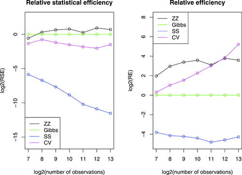
Fig. 3 Dynamics of the samplers on a robust regression example with spike and slab or horseshoe prior. The top row shows the posterior for θ₁ and θ₂, bottom row shows the estimates for θ₂ and θ₃. The spike-and-slab distributions are sampled using the reversible jump PDMP samplers with reversible jump parameter 0.6 and refreshment for the BPS methods set to 0.5. All methods are shown with 10³ samples (red) and the PDMP dynamics are shown in black. Sampling with the Horseshoe prior was implemented in Stan using NUTS. Both Stan and PDMP methods were run for the same computing time. To aid visualization only the first 30% of the PDMP trajectories are shown.

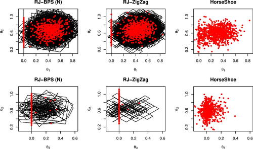
Fig. 4 Sampling efficiency for reversible jump PDMP versus Stan for the robust regression example. The PDMP samplers are ZigZag (zz), Bouncy Particle Sample with normally distributed velocities (bps_n) and with velocities distributed uniformly on the sphere (bps_s). The top figure shows boxplots of the posterior mean of θ₁ for increasing computational budget, with outliers from the sampler removed for visualization purposes. These removed outliers correspond to times that the sampler has become stuck in a local mode where ${\theta }_1=0$. The subplot shows the full results including outliers from the samplers. The Stan sampler is sampling from a different posterior to the PDMP methods, and this is seen in the estimates converging to slightly different values; but Monte Carlo efficiency can be assessed by comparing the variability of the estimates. The bottom figure shows the number of times that the samplers did not find the global mode.

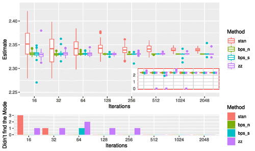
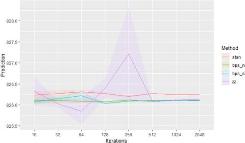
Fig. 5 Predictive ability of reversible jump PDMP versus Stan for the robust regression example. The PDMP samplers are ZigZag (zz), Bouncy Particle Sample with normally distributed velocities (bps_n) and with velocities distributed uniformly on the sphere (bps_s). The predictive ability is measured by Monte Carlo estimates of the mean square predictive performance.