Poisson-FOCuS: An Efficient Online Method for Detecting Count Bursts with Application to Gamma Ray Burst Detection

Figures & data

Fig. 1 Plots of two recorded gamma ray bursts from the FERMI GBM Burst catalogue, with photon counts binned into 0.2 sec and 2 sec intervals.

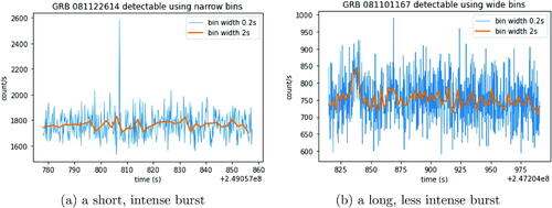
Fig. 2 Example 4 hr of background data from one detector, grouped into 10 sec bins to show background rate fluctuations.

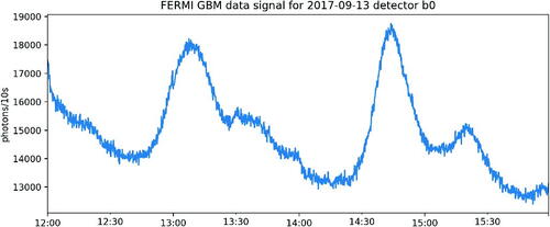
Fig. 3 A schematic of the detection system, with the arrow thickness corresponding to the relative velocities of data flows. Most of the computing requirements of the trigger algorithm are within the detection loop, highlighted in green.

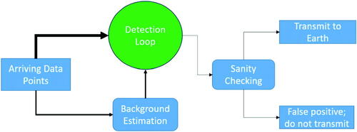
Fig. 4 A simulated example anomaly with intensity multiplier μ = 3 and duration h = 20 against a background λ = 2.

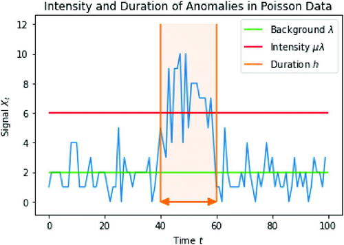
Fig. 5 Detectability of GRBs at different k-sigma levels. Shaded regions show values of $h\lambda$ and ${\widehat{\mu }}_{t+1:t+h}$ where the likelihood ratio exceeds k-sigma event thresholds for k = 3 (blue region), k = 5 (orange region) and k = 7 (green region) for a test that uses the correct value of h.

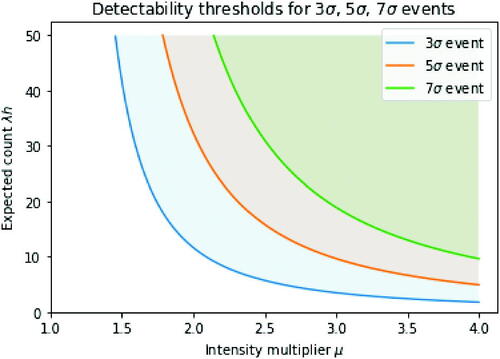
Fig. 6 Detectability of GRBs by the window method, for one window (left) or a grid of three windows (right). The orange shaded area shows the values of $h\lambda$ and ${\widehat{\mu }}_{t+1:t+h}$ where the likelihood ratio exceeds a 5-sigma threshold, and the blue shaded area shows the detectability region form Figure 5. Dashed lines show expected count $h\lambda$ over the window.

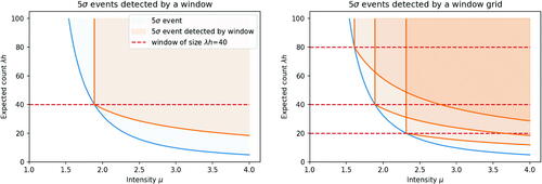
Fig. 7 Detectability of GRBs by Page-CUSUM for a single μ value (left) and a grid of three μ values (right). Orange shaded area shows the values of $h\lambda$ and ${\widehat{\mu }}_{t+1:t+h}$ where the likelihood ratio exceeds a 5-sigma threshold; the green shaded area shows the detectability region for the corresponding window test as defined by Proposition 2 (left-hand plot); and the blue shaded area shows the detectability region from Figure 5.

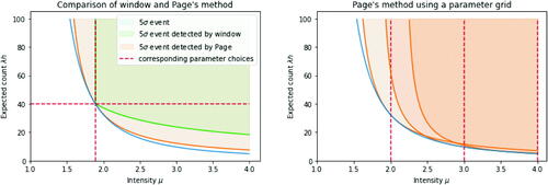
Fig. 8 Three example logarithmic curves. The statistic $S_T(\mu )$ is defined as the maximum of all logarithmic curves and the 0 line.

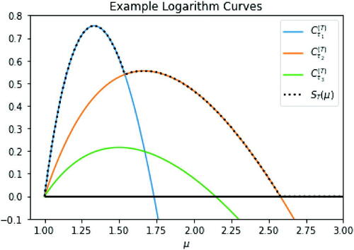
Fig. 9 Comparisons of the number of windows and expected number of curves (average over 1000 runs) kept by FOCuS running over a signal with base rate λ = 100 using a 5-sigma threshold, with no constraint on length of GRB (left) and with $h_{\max }=1024$, corresponding to ${\mu }_{\min }=1.02$ (right).

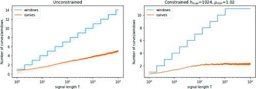
Fig. 10 Comparison between FOCuS and logarithmic window method showing the average run length at different sigma levels.

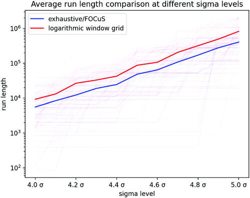
Fig. 11 Plots of runs of FOCuS and window-based method on simulated GRB copies of different brightnesses. Left-hand column shows three example GRBs each simulated to have 1000 photons. Right-hand column shows corresponding largest value of the test statistic as a function of number of photons in GRB. In plot (f) the lines for the two methods almost perfectly overlay one another.

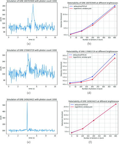
Fig. 12 An hour’s portion of the same data from Figure 2 at higher resolution of 50ms (blue). In black is the data at 10 sec resolution identical to that from Figure 2 but rescaled by 0.005x to fit the graph. In orange is a centered 3 min moving-average background estimate (linewidth increased for visual clarity).

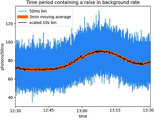
Fig. 13 Plots of a run of FOCuS over the data using various background estimation methods and parameters: (a) using a unbiased estimator of the background rate; (b) using a biased estimator; (c) using the same biased estimator but with ${\mu }_{\min }=1.1$.

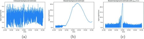
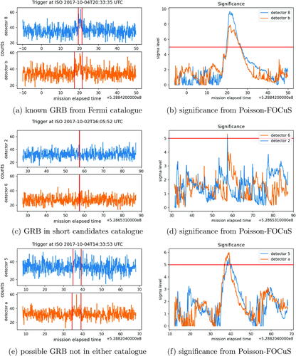
Fig. 14 Three of the triggers found in the FERMI daily data. Left-hand column shows data from the two detectors that give a trigger, and the right-hand column shows the corresponding output from the Poisson-FOCuS algorithm.

Data Availability Statement

Code for Poisson-FOCuS and the analysis for this article is available at the GitHub repository https://github.com/kesward/FOCuS.