Data Fission: Splitting a Single Data Point

Figures & data

Fig. 1 Illustration of typical data splitting procedures for post-selection inference. Splitting the data has the advantage of allowing the user to choose any selection strategy for model selection, but at the cost of decreased power during the inference stage.

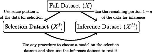
Fig. 2 Illustration of the proposed data fission procedure. Similar to data splitting, it allows for any selection procedure for choosing the model. However, it achieves this through randomization rather than a direct splitting of the data.

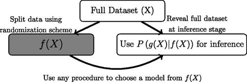
Fig. 3 Illustration of data carving procedure as discussed in Fithian, Sun, and Taylor (2014). Data carving has the advantage of using all unused information for inference, but requires the selection procedure to be fixed at the onset of investigation. Moreover, computing the conditional distribution needs to be tractable, either in closed form (e.g., LASSO as described in Lee et al. 2016) or through numerical simulation. Thus, data carving and fission have complementary benefits and tradeoffs.

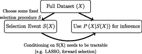
Fig. 4 Numerical results averaged over 250 trials for a $50\times 50$ grid of hypotheses with target FDR level chosen at 0.2 and τ varying over (0, 1). Solid lines denote metrics for the rejection sets formed using the full dataset and dotted lines denote metrics calculated using the rejection sets formed through data fission. All methods control FDR at the desired level, but “double dipping” to form CIs after forming a rejection set data results in invalid coverage. Fissioned CIs have the correct coverage. The fissiones CI lengths decrease as τ increases because more of the dataset gets reserved for inference.

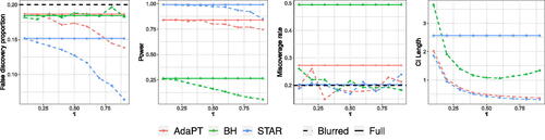
Fig. 5 Comparison of data splitting (left) and data fission (middle, right) for dataset with one highly influential point. Splitting the data and fitting a regression results in substantially different fitted models because the fitted values are heavily influenced by a single data point. In contrast, data fission keeps the same X location for every data point, but randomly perturbs the response Y with random noise to create new variables f(Y) and g(Y): notice the slight difference in the two figures. This enables the analyst to keep a “piece” of every data point in both f(Y) and g(Y), ensuring that leverage points have an impact in both copies of the dataset.

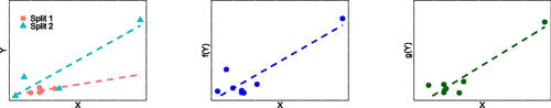
Fig. 6 An instance of the selected feature (blue crosses) and the constructed CIs using fissioned data (left), full data twice (middle), and split data (right) with $S_{\Delta }=0.2$ and target FCR set at 0.2. The selected features are marked by blue crosses, which include all of the nonzero coefficients (corresponding to almost 100% power for selection) and also a few zero coefficients (corresponding to around 70% precision for selection). CIs which do not cover the parameters correctly are marked red.

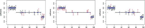
Fig. 7 FCR, average length of the CIs, and power/precision for the selected features, when varying the leverage parameter γ in $\{2,3,4,5,6\}$. The results are averaged over 500 trials. Both data splitting and data fission still control FCR, but data fission now has higher power and precision, as well as tighter CIs than data splitting.

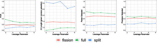
Fig. 8 FCR, length of the CIs, FSR, power for the sign of parameters, and power and precision for the selected features, when varying the leverage parameter α in $\{2,3,4,5,6\}$ for Poisson data over 500 trials. CIs constructed using data fission are tighter than data splitting, and power during the selection stage is higher.

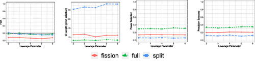
Fig. 9 Two instances of the observed points (in yellow) and the pointwise CIs (in blue if correctly cover the trend, in red if not; the time points with false coverage are also amplified in the bar at the bottom) using two types of methods: full data twice (left), and data fission (right). The underlying projected mean is marked in cyan, which mostly overlaps with the true underlying trend. The true knots are marked by vertical lines. Using data fission results in correct empirical coverage (the 0.225 above was for just one run, the average is below 0.2). In contrast, the FCR is not controlled when using the full dataset twice; it worsens as the underlying noise and trend become more volatile.

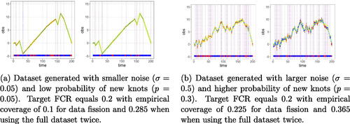
Fig. 10 FCR for the pointwise CIs and simultaneous Type I error for uniform CIs when varying the probability of having knots p in $\{0.01,0.55,0.1,0.145,0.19\}$ and the noise SD in $\{0.05,0.1,0.15,0.2\}$ (the blue circled cell represents the setting for the first shown instance in Figure 9). The CIs generated using full data twice do not have valid FCR or simultaneous Type I error control, especially when p is large (more knots) and the noise standard deviation is small, but data fission is always valid.

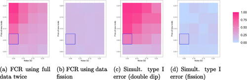
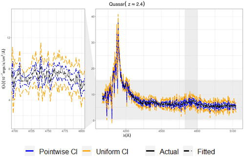
Fig. 11 Fitted values as well as uniform and pointwise CIs for a quasar object fit using linear trend filtering. The right view shows the trend filter over the entire spectrum, but the left view “zooms in” on a smaller subset of the data to aid in visual identification.

Fithian, W., Sun, D., and Taylor, J. (2014), “Optimal Inference after Model Selection,” arXiv:1410.2597.

 Google Scholar

Lee, J. D., Sun, D. L., Sun, Y., and Taylor, J. E. (2016), “Exact Post-Selection Inference, with Application to the Lasso,” The Annals of Statistics, 44, 907–927. DOI: 10.1214/15-AOS1371.

 Web of Science ®Google Scholar