Latent Space Modeling of Hypergraph Data

Figures & data

Fig. 1 Examples of hypergraph datasets. (b) shows co-tagging data and (c) shows a subsample of the coauthorship network of Ji and Jin (2016). The figures were made with R packages HyperG (Marchette 2021) and igraph (Csardi and Nepusz 2006).

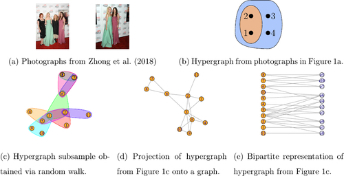
Fig. 2 Example of a Čech complex. Left: $B_r(u_i)$ for ${\{u_i=(u_{i1},u_{i2})\}}_{i=1}^7$ in ${\mathbb{R}}^2$. Middle: the graph obtained by taking pairwise intersections. Right: the hypergraph obtained by taking intersections of arbitrary order. The shaded region indicates an order 3 hyperedge.

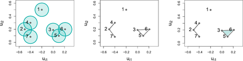
Fig. 3 Example of a nsRGH (see Definition 3.1) with $\mathit{U}={\left\{u_i\right\}}_{i=1}^7={\{(u_{i1},u_{i2})\}}_{i=1}^7$. Left: ${\mathcal{C}}_{r_2}(\mathit{U})$. Middle: ${\mathcal{C}}_{r_3}(\mathit{U})$. Right: ${\cup }_{k=2}^3{\mathcal{D}}_{r_k}^{(k)}(\mathit{U})$.

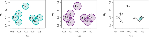
Fig. 4 Comparison of theoretical (solid) and Monte Carlo (dashed) estimates of $p(y_{e_{k,i}}^{(g)}=1|u_i,r_k,\mu ,\Sigma )$ for varying r_k . We take $\Sigma =\text{diag}(1,1),\mu =(0,0)$ and consider connection probabilities for k = 2, 3, 4. In the left plot $u_i=\mu$ and in the right plot $u_i=(1,2)$. The same study with $\Sigma =\text{diag}(1,2)$ is provided in Supplement F.3.

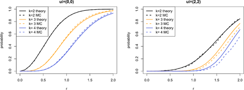
Fig. 5 Comparison between empirical (dashed line) and Poisson approximation (points) of the order k = 3 degree distribution conditional on the latent coordinate u_i . We take $N=10,\mu =(0,0),\Sigma =\text{diag}(1,1)$ and evaluate the distribution for $r_3\in (0.1,0.4,1.0)$. The left plot shows $u_i=\mu$ and the right plot shows $u_i=(1,2)$. The equivalent Figures with $\Sigma =\text{diag}(1,2)$ and N = 20 are given in Supplement F.3.

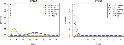
Fig. 6 Comparison of true and posterior predictive degree distributions for hyperedges of order k = 2 (left) and k = 3 (right). Vertical lines and black dots correspond to the range and median of the probabilities of observing each degree as calculated via the posterior predictive. The observed degree is shown as green triangles.

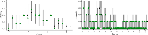
Fig. 7 Summary of average per-iteration costs after 200 iterations for an MCMC implemented with and without delayed acceptance (DA) for 10 datasets sampled from data regimes (R1) (black, circle) and (R2) (red, triangle). Left: average per-iteration cost in seconds for a DA scheme. Right: ratio of average per-iteration cost for a DA scheme and a scheme without DA. Numbers less than 1 imply DA offers a computational speed-up.

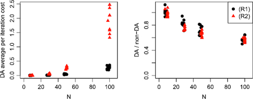
Fig. 8 Visualization of the datasets considered in Section 7. The hyperedges correspond to the observations for each dataset. Each figure shows the full hypergraph (left) and a subset sampled according to a random walk (right).

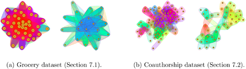
Fig. 9 Summary of predictive distributions for $N^{*}$ additional nodes for the Grocery dataset. For each measure we report the proportion of predictions which are distance D from the truth, where D is the absolute difference between the predictive and the truth.

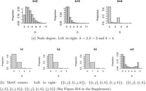
Fig. 10 Summary of predictive distributions for $N^{*}$ additional nodes for the coauthorship dataset. For each measure we report the proportion of predictions which are distance D from the truth, where D is the absolute difference between the predictive and the truth.

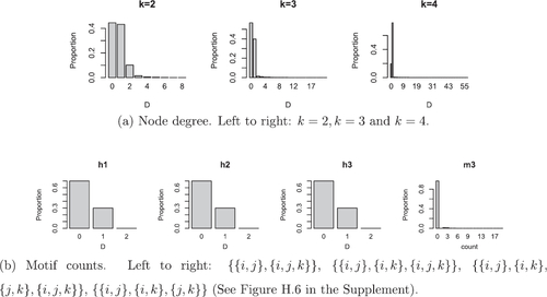
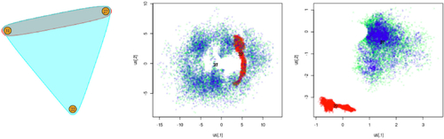
Fig. 11 Comparison between latent positions for subset of the coauthorship network on nodes {22, 27, 31}. Left: observed interactions. Middle: traceplot of latent positions for model with r_k = r. Right: traceplot of latent positions for our model with $r_k>r_{k-1}$.

Ji, P., and Jin, J. (2016), “Coauthorship and Citation Networks for Statisticians,” The Annals of Applied Statistics, 10, 1779–1812. DOI: 10.1214/15-AOAS896.

 Web of Science ®Google Scholar

Marchette. (2021), HyperG: Hypergraphs in R, R package version 1.0.0.

 Google Scholar

Csardi, G., and Nepusz, T. (2006), “The igraph Software Package for Complex Network Research,” InterJournal, complex systems, 1695.5, 1–9.

 Google Scholar