Coexchangeable Process Modeling for Uncertainty Quantification in Joint Climate Reconstruction

Figures & data

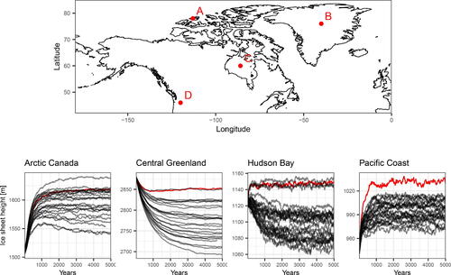
Fig. 1 Graphical representation of the coexchangeable and coexchangeable process models. Boxes represent observed quantities, dashed circles represent unobserved quantities over which we make prior belief specifications, and solid circles represent unobserved quantities for which we calculate updated beliefs. Analogous to conditional independence in probabilistic models, arrows may be used to identify Bayes linear sufficiency between quantities. For simplicity, residual terms are omitted.

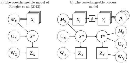
Fig. 2 Proxy-based measurements of LGM SST and maximum sea-ice extents. Annual and summer mean SST’s are represented by points and triangles, respectively. Sea-ice extents are represented by a red dashed line. The Southern sea-ice extent is as reported in Gersonde et al. (2005) and the Northern sea-ice extent is provided by coauthors.

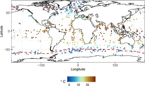
Fig. 3 Adjusted beliefs of January SST: (a) expectation of SST adjusted by $\overline{\mathbf{X}}$, equal to the ensemble mean; (b) marginal standard deviation of SST adjusted by $\overline{\mathbf{X}}$; (c) expectation of SST adjusted by $\overline{\mathbf{X}}$ and ${\mathbf{Z}}_{\mathbf{X}}$; (d) marginal standard deviation of SST adjusted by $\overline{\mathbf{X}}$ and ${\mathbf{Z}}_{\mathbf{X}}$; (e) contribution of the data to our expected beliefs of SST ${\mathbb{E}}_{\overline{\mathbf{X}},{\mathbf{Z}}_{\mathbf{X}}}[{\mathbf{X}}^{*}]-\overline{\mathbf{X}}$; and (f), marginal standard deviation of the ensemble. All plots are shown in degrees Celsius.

Fig. 4 Spline fits, parameterized by ${\mathit{\beta }}^i$, of SIC given SST to each ensemble member prior to the coexchangeable adjustment. Shaded regions denote ±2 standard deviations.

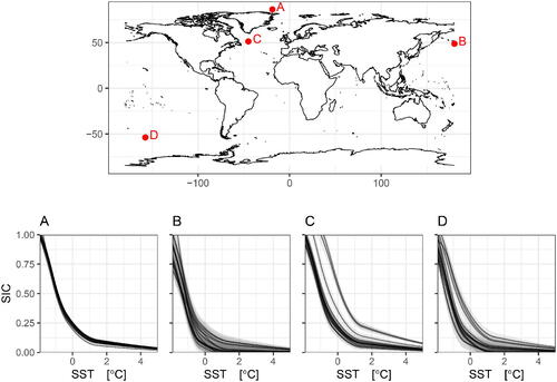
Fig. 5 Adjusted beliefs of August SIC given expected SST, ${\mathbf{X}}^{*}={\mathbb{E}}_{\overline{\mathbf{X}},{\mathbf{Z}}_{\mathbf{X}}}[{\mathbf{X}}^{*}]$: (a) expectation of SIC adjusted by $\widehat{\mathit{\beta }}$; (b) marginal standard deviation of SIC adjusted by $\widehat{\mathit{\beta }}$; (c) expectation of SIC adjusted by $\widehat{\mathit{\beta }}$ and ${\mathbf{Z}}_{\mathbf{Y}}$; (d) marginal standard deviation of SIC adjusted by $\widehat{\mathit{\beta }}$ and ${\mathbf{Z}}_{\mathbf{Y}}$; (e) ensemble mean; and (f), marginal standard deviation of the ensemble. Values are of sea-ice concentration measured between 0 and 1.

Fig. 6 A single plausible sample from the SST and SIC reconstructions. (a) and (b) show SSTs from February and August, respectively and (c) and (d) show SICs from February and August, respectively.

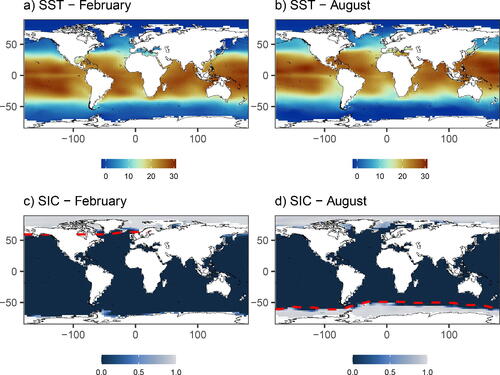
Fig. 7 Ensemble time-series plots at four spatial locations: Arctic Canada (A), Central Greenland (B), Hudson Bay (C), and the Pacific Coast (D). The reference run is shown in red, the simulations forced with sampled boundary conditions in black.

Gersonde, R., Crosta, X., Abelmann, A., and Armand, L. (2005), “Sea-Surface Temperature and Sea Ice Distribution of the Southern Ocean at the EPILOG Last Glacial Maximum–a circum-Antarctic view based on Siliceous Microfossil Records,” Quaternary Science Reviews, 24, 869–896. DOI: 10.1016/j.quascirev.2004.07.015.

 Web of Science ®Google Scholar